Tutorial 1: Introduction to braintools.input

Welcome to the braintools.input tutorial series! This module provides comprehensive tools for generating current inputs used in computational neuroscience simulations.

Learning Objectives

By the end of this tutorial, you will:

• Understand what current inputs are and their role in neuroscience

• Learn the difference between Composable and Functional APIs

• Set up your environment for braintools

• Generate your first current inputs

• Create basic visualizations of current signals

1. What are Current Inputs?

Current inputs are electrical stimuli applied to neurons or neural models to study their behavior. They are fundamental in:

• Electrophysiology: Injecting current through patch pipettes

• Optogenetics: Light-activated current generation

• Neural stimulation: Deep brain stimulation, TMS, etc.

• Computational modeling: Simulating synaptic inputs and external stimuli

Types of Current Inputs

• Basic patterns: Constant, step, ramp currents

• Periodic waveforms: Sine waves, square waves, chirps

• Pulse patterns: Spikes, bursts, synaptic-like pulses

• Stochastic inputs: Noise, random processes

2. Environment Setup

Let’s start by importing the necessary libraries and setting up our environment.

# Essential imports
import numpy as np
import matplotlib.pyplot as plt
import brainstate
import brainunit as u
import braintools

# Set up plotting
plt.style.use('default')
plt.rcParams['figure.figsize'] = (10, 6)
plt.rcParams['font.size'] = 12

3. Two APIs Overview

braintools.input provides two complementary APIs:

Composable API (Object-Oriented)

• Recommended for complex protocols

• Inputs are objects that can be combined and transformed

• Supports operations like addition, multiplication, clipping

• More flexible and powerful

Functional API (Traditional)

• Good for simple, direct array generation

• Functions that directly return arrays

• Familiar to users of scipy.signal

• More straightforward for basic use cases

4. Setting Up the Simulation Environment

Before generating any inputs, we need to set up the temporal resolution using brainstate’s environment context.

# Set the time step for our simulations
dt = 0.1 * u.ms  # 100 microseconds - good resolution for most applications

print(f"Time step: {dt}")
print(f"This means 1 ms contains {int(1 * u.ms / dt)} time points")

Time step: 0.1 * msecond
This means 1 ms contains 10 time points

5. Your First Current Inputs

Let’s generate some basic current patterns using both APIs.

5.1 Constant Current

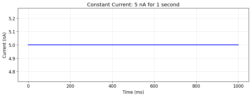
# Using Composable API
with brainstate.environ.context(dt=dt):
    # Create a constant current of 5 nA for 1 second
    constant_composable = braintools.input.Constant([(5.0, 1000 * u.ms)])
    signal_composable = constant_composable()

# Using Functional API  
with brainstate.environ.context(dt=dt):
    signal_functional = braintools.input.constant([(5.0, 1000 * u.ms)])[0]

print(f"Composable signal shape: {signal_composable.shape}")
print(f"Functional signal shape: {signal_functional.shape}")
print(f"Signals are equal: {np.allclose(u.get_magnitude(signal_composable), u.get_magnitude(signal_functional))}")

Composable signal shape: (10000,)
Functional signal shape: (10000,)
Signals are equal: True

# Let's plot the constant current
def plot_signal(signal, duration, title, ax=None):
    """Helper function to plot current signals."""
    if ax is None:
        fig, ax = plt.subplots(figsize=(10, 4))

    # Create time axis
    dt_val = u.get_magnitude(dt)
    duration_val = u.get_magnitude(duration)
    time_points = np.arange(0, duration_val, dt_val)

    # Get signal magnitude
    signal_val = u.get_magnitude(signal)

    ax.plot(time_points, signal_val, 'b-', linewidth=2)
    ax.set_xlabel('Time (ms)')
    ax.set_ylabel('Current (nA)')
    ax.set_title(title)
    ax.grid(True, alpha=0.3)

    return ax


# Plot the constant current
plot_signal(signal_composable, 1000 * u.ms, 'Constant Current: 5 nA for 1 second')
plt.tight_layout()
plt.show()

5.2 Ramp Current

# Create a ramp from 0 to 10 nA over 500 ms
with brainstate.environ.context(dt=dt):
    # Composable API
    ramp_composable = braintools.input.Ramp(0, 10, 500 * u.ms)
    ramp_signal_comp = ramp_composable()

    # Functional API
    ramp_signal_func = braintools.input.ramp(0, 10, 500 * u.ms)

# Plot both signals
fig, (ax1, ax2) = plt.subplots(2, 1, figsize=(10, 8))

plot_signal(ramp_signal_comp, 500 * u.ms, 'Ramp Current (Composable API)', ax1)
plot_signal(ramp_signal_func, 500 * u.ms, 'Ramp Current (Functional API)', ax2)

plt.tight_layout()
plt.show()

print(f"Maximum difference between APIs: {np.max(np.abs(u.get_magnitude(ramp_signal_comp - ramp_signal_func))):.2e} nA")

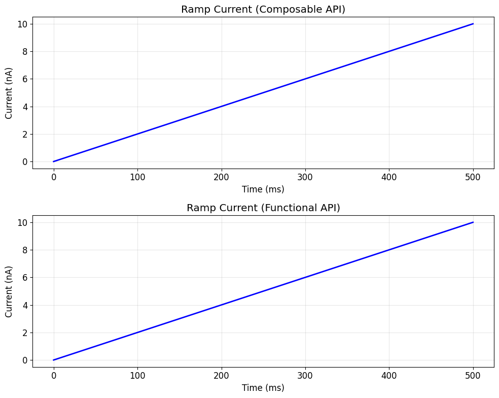
Maximum difference between APIs: 0.00e+00 nA

5.3 Step Current

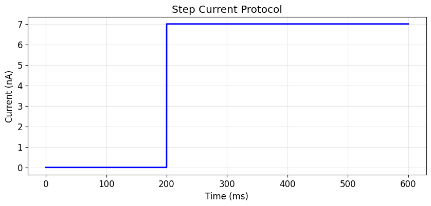
# Create a step current: 0 → 3 → 7 → 0 nA
with brainstate.environ.context(dt=dt):
    step_current = braintools.input.Step(
        [0, 3, 7, 0],
        [100 * u.ms, 200 * u.ms, 200 * u.ms, 100 * u.ms],
        duration=600 * u.ms
    )
    step_signal = step_current()

plot_signal(step_signal, 600 * u.ms, 'Step Current Protocol')
plt.show()

6. Basic Waveforms

6.1 Sinusoidal Current

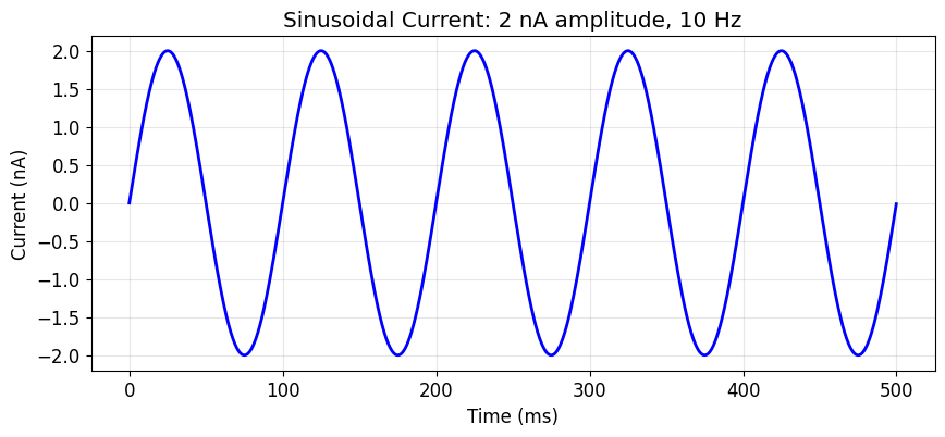
# Generate a 10 Hz sinusoidal current
with brainstate.environ.context(dt=dt):
    sine_current = braintools.input.Sinusoidal(amplitude=2.0, frequency=10 * u.Hz, duration=500 * u.ms)
    sine_signal = sine_current()

plot_signal(sine_signal, 500 * u.ms, 'Sinusoidal Current: 2 nA amplitude, 10 Hz')
plt.show()

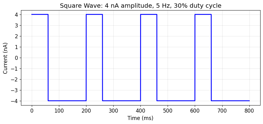
6.2 Square Wave Current

# Generate a 5 Hz square wave with 30% duty cycle
with brainstate.environ.context(dt=dt):
    square_current = braintools.input.Square(amplitude=4.0, frequency=5 * u.Hz, duration=800 * u.ms, duty_cycle=0.3)
    square_signal = square_current()

plot_signal(square_signal, 800 * u.ms, 'Square Wave: 4 nA amplitude, 5 Hz, 30% duty cycle')
plt.show()

7. Understanding Parameters and Units

braintools.input uses brainunit for proper unit handling. This ensures dimensional consistency and prevents common errors.

# Examples of different units
print("Time units:")
print(f"1 second = {1 * u.second}")
print(f"500 milliseconds = {500 * u.ms}")
print(f"100 microseconds = {100 * u.us}")

print("\nCurrent units:")
print(f"1 nanoamp = {1 * u.nA}")
print(f"1 picoamp = {1 * u.pA}")
print(f"0.5 microamp = {0.5 * u.uA}")

print("\nFrequency units:")
print(f"10 Hz = {10 * u.Hz}")
print(f"1 kHz = {1 * u.kHz}")

Time units:
1 second = 1 * second
500 milliseconds = 500 * msecond
100 microseconds = 100 * usecond

Current units:
1 nanoamp = 1 * namp
1 picoamp = 1 * pamp
0.5 microamp = 0.5 * uamp

Frequency units:
10 Hz = 10 * hertz
1 kHz = 1 * khertz

# Example: Creating currents with different amplitudes and units
with brainstate.environ.context(dt=dt):
    # Small current in picoamps
    small_current = braintools.input.Constant([(100 * u.pA, 200 * u.ms)])
    small_signal = small_current()

    # Medium current in nanoamps
    medium_current = braintools.input.Constant([(2 * u.nA, 200 * u.ms)])
    medium_signal = medium_current()

    # Large current in microamps
    large_current = braintools.input.Constant([(0.01 * u.uA, 200 * u.ms)])
    large_signal = large_current()

# Plot all three
fig, axes = plt.subplots(3, 1, figsize=(10, 10))

plot_signal(small_signal, 200 * u.ms, 'Small Current: 100 pA', axes[0])
plot_signal(medium_signal, 200 * u.ms, 'Medium Current: 2 nA', axes[1])
plot_signal(large_signal, 200 * u.ms, 'Large Current: 0.01 μA = 10 nA', axes[2])

plt.tight_layout()
plt.show()

print(
    f"All currents in nA: {u.get_magnitude(small_signal[0]):.3f}, {u.get_magnitude(medium_signal[0]):.3f}, {u.get_magnitude(large_signal[0]):.3f}")

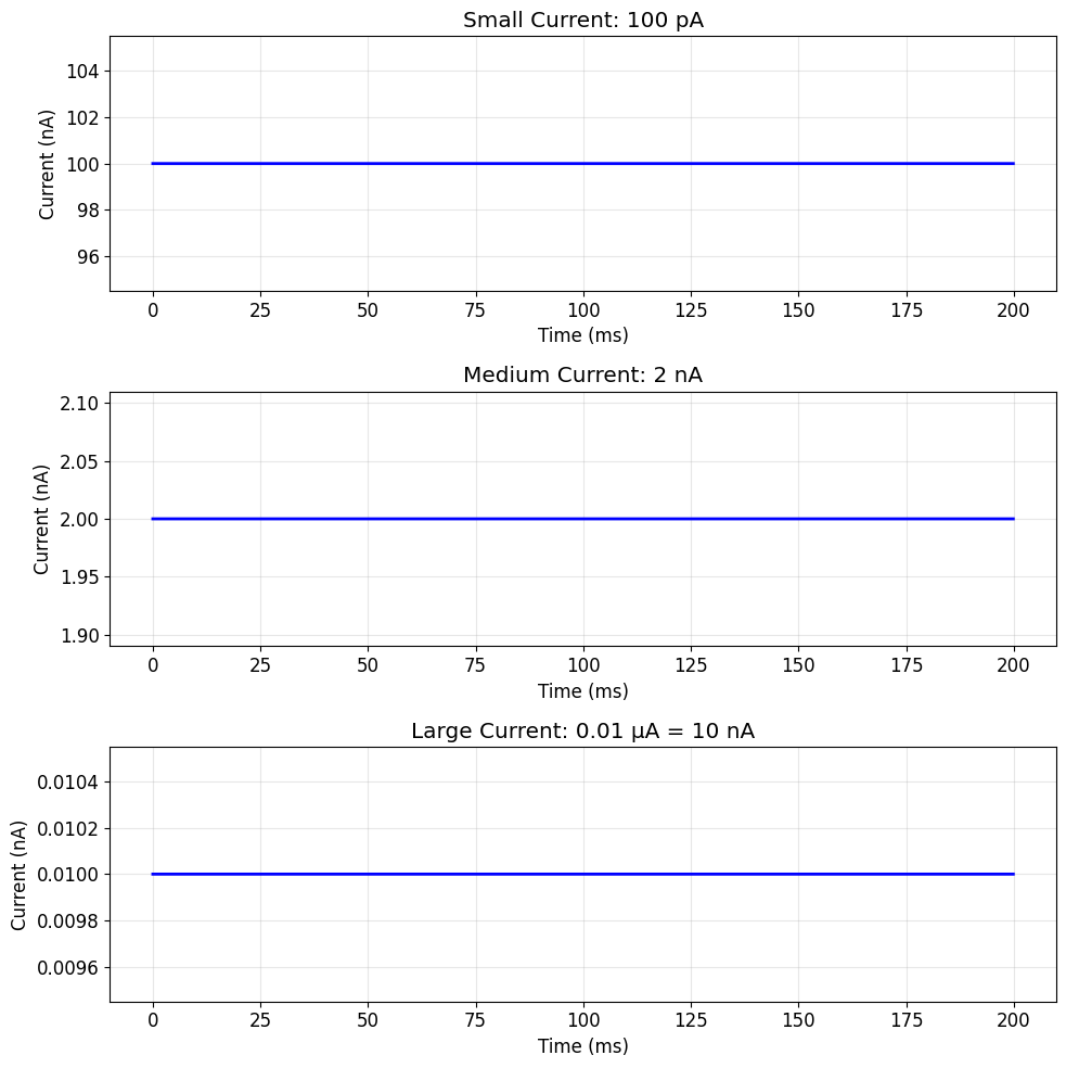
All currents in nA: 100.000, 2.000, 0.010

9. Key Concepts Summary

What we learned:

1. Current inputs are fundamental tools in neuroscience for stimulating neurons and neural circuits

2. Two APIs available:

   • Composable API: Object-oriented, more powerful for complex protocols

   • Functional API: Simple function calls, good for basic use

3. Essential setup:

   • Always use brainstate.environ.context(dt=...) to set temporal resolution

   • Use brainunit for proper unit handling

4. Basic input types:

   • Constant: Sustained current levels

   • Step: Instantaneous current changes

   • Ramp: Linear current transitions

   • Section: Multi-phase protocols

   • Sinusoidal: Rhythmic oscillations

   • Square: Pulse-like patterns

5. Units matter: Always specify proper units (nA, ms, Hz) to avoid errors

10. Practice Exercises

Try these exercises to reinforce your learning:

# Exercise 1: Create a 2-second constant current of 3 nA
# Your code here:

with brainstate.environ.context(dt=dt):
    # TODO: Create constant current
    pass

# Uncomment to test:
# plot_signal(your_signal, 2000*u.ms, 'Exercise 1: 3 nA constant current')
# plt.show()

# Exercise 2: Create a ramp from -5 to 5 nA over 500 ms
# Your code here:

with brainstate.environ.context(dt=dt):
    # TODO: Create ramp
    pass

# Uncomment to test:
# plot_signal(your_ramp, 500*u.ms, 'Exercise 2: -5 to 5 nA ramp')
# plt.show()

# Exercise 3: Create a 20 Hz sinusoidal current with 1.5 nA amplitude for 300 ms
# Your code here:

with brainstate.environ.context(dt=dt):
    # TODO: Create sinusoidal current
    pass

# Uncomment to test:
# plot_signal(your_sine, 300*u.ms, 'Exercise 3: 20 Hz sinusoid')
# plt.show()

Solutions (Run after attempting exercises)

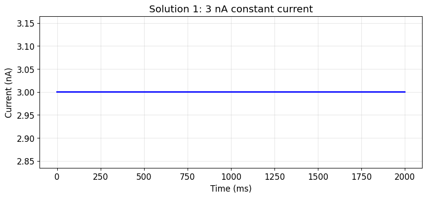
# Solution 1
with brainstate.environ.context(dt=dt):
    ex1_current = braintools.input.Constant([(3.0, 2000 * u.ms)])
    ex1_signal = ex1_current()

plot_signal(ex1_signal, 2000 * u.ms, 'Solution 1: 3 nA constant current')
plt.show()

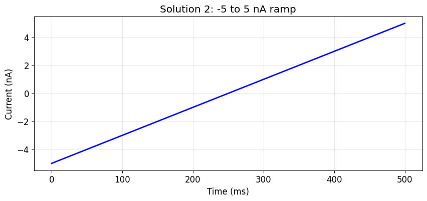
# Solution 2
with brainstate.environ.context(dt=dt):
    ex2_ramp = braintools.input.Ramp(-5, 5, 500 * u.ms)
    ex2_signal = ex2_ramp()

plot_signal(ex2_signal, 500 * u.ms, 'Solution 2: -5 to 5 nA ramp')
plt.show()

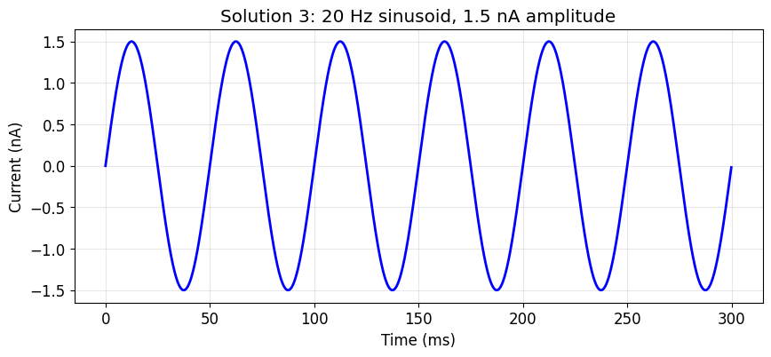
# Solution 3
with brainstate.environ.context(dt=dt):
    ex3_sine = braintools.input.Sinusoidal(1.5, 20 * u.Hz, 300 * u.ms)
    ex3_signal = ex3_sine()

plot_signal(ex3_signal, 300 * u.ms, 'Solution 3: 20 Hz sinusoid, 1.5 nA amplitude')
plt.show()

Next Steps

Now that you understand the basics, you can move on to:

• Tutorial 2: Functional APIs - Deep dive into the functional approach with all input types

• Tutorial 3: Composable APIs - Learn to combine and transform inputs for complex protocols

• Tutorial 4: Custom Transformations and Pipelines - Advanced techniques for real-world applications

Great job completing your first braintools.input tutorial! 🎉