MultiGaussianGrad

MultiGaussianGrad#

class braintools.surrogate.MultiGaussianGrad(h=0.15, s=6.0, sigma=0.5, scale=0.5)#

Judge spiking state with the multi-Gaussian gradient function [1].

The Multi-Gaussian gradient surrogate combines three Gaussian components to create a more complex gradient profile. It uses a positive central Gaussian and two negative side Gaussians, allowing for enhanced gradient flow and potentially better training dynamics in spiking neural networks.

The forward function:

\[\begin{split}g(x) = \begin{cases} 1, & x \geq 0 \\ 0, & x < 0 \\ \end{cases}\end{split}\]

Backward gradient:

\[g'(x) = \text{scale} \cdot \left[ (1+h) \cdot \mathcal{N}(x; 0, \sigma^2) - h \cdot \mathcal{N}(x; \sigma, (s\sigma)^2) - h \cdot \mathcal{N}(x; -\sigma, (s\sigma)^2) \right]\]

where \(\mathcal{N}(x; \mu, \sigma^2)\) is the Gaussian PDF with mean μ and variance σ².

The gradient consists of:

A central positive Gaussian at x=0 with weight (1+h)
Two negative side Gaussians at x=±σ with weight -h
Side Gaussians have wider spread controlled by parameter s

>>> import jax
>>> import jax.numpy as jnp
>>> import brainstate
>>> import braintools.surrogate as surrogate
>>> import matplotlib.pyplot as plt
>>>
>>> xs = jnp.linspace(-3, 3, 1000)
>>> fig, (ax1, ax2) = plt.subplots(1, 2, figsize=(10, 4))
>>>
>>> # Plot default multi-Gaussian gradient
>>> mgg_fn = surrogate.MultiGaussianGrad()
>>> grads = jax.vmap(jax.grad(mgg_fn))(xs)
>>> ax1.plot(xs, grads, label='Multi-Gaussian', linewidth=2)
>>>
>>> # Compare with single Gaussian
>>> gg_fn = surrogate.GaussianGrad(sigma=0.5, alpha=0.5)
>>> grads_single = jax.vmap(jax.grad(gg_fn))(xs)
>>> ax1.plot(xs, grads_single, '--', label='Single Gaussian', alpha=0.7)
>>>
>>> ax1.set_xlabel('Input (x)')
>>> ax1.set_ylabel('Gradient')
>>> ax1.set_title('Multi-Gaussian vs Single Gaussian')
>>> ax1.legend()
>>> ax1.grid(True, alpha=0.3)
>>> ax1.axhline(y=0, color='k', linestyle='-', linewidth=0.5)
>>>
>>> # Show effect of h parameter (side peak weight)
>>> for h in [0.0, 0.15, 0.3, 0.5]:
>>>     mgg_fn = surrogate.MultiGaussianGrad(h=h, s=6.0, sigma=0.5, scale=0.5)
>>>     grads = jax.vmap(jax.grad(mgg_fn))(xs)
>>>     ax2.plot(xs, grads, label=rf'$h={h}$')
>>>
>>> ax2.set_xlabel('Input (x)')
>>> ax2.set_ylabel('Gradient')
>>> ax2.set_title('Effect of h Parameter')
>>> ax2.legend()
>>> ax2.grid(True, alpha=0.3)
>>> ax2.axhline(y=0, color='k', linestyle='-', linewidth=0.5)
>>> plt.tight_layout()
>>> plt.show()

(Source code, png, hires.png, pdf)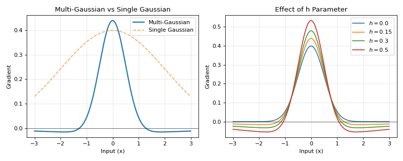

../../_images/braintools-surrogate-MultiGaussianGrad-1.png

Parameters:

h (float, optional) – Weight parameter for side Gaussians. Default is 0.15. Controls the depth of negative side lobes.
s (float, optional) – Width scaling factor for side Gaussians. Default is 6.0. Larger values make side Gaussians wider.
sigma (float, optional) – Standard deviation of central Gaussian and position of side peaks. Default is 0.5.
scale (float, optional) – Overall gradient scaling factor. Default is 0.5.

Examples

>>> import jax
>>> import braintools.surrogate as surrogate
>>>
>>> # Create multi-Gaussian gradient surrogate
>>> mgg_fn = surrogate.MultiGaussianGrad(h=0.15, s=6.0, sigma=0.5, scale=0.5)
>>>
>>> # Apply to input
>>> x = jax.numpy.array([-1., -0.5, 0., 0.5, 1.])
>>> spikes = mgg_fn(x)
>>> print(spikes)
[0. 0. 1. 1. 1.]
>>>
>>> # Compute gradients showing multi-peak structure
>>> grad_fn = jax.grad(lambda x: mgg_fn(x).sum())
>>> grads = grad_fn(x)
>>> print(f"Gradients: {grads}")

MultiGaussianGrad

Contents

MultiGaussianGrad#