Tutorial 1: Basic Weight Initialization Distributions

Tutorial 1: Basic Weight Initialization Distributions#

This tutorial introduces the fundamental weight initialization distributions available in BrainTools. Weight initialization is crucial for training neural networks effectively, as poor initialization can lead to vanishing/exploding gradients, slow convergence, or inability to learn.

Topics Covered#

Introduction to weight initialization
Constant, Uniform, and Normal distributions
Statistical distributions: LogNormal, Gamma, Exponential, Weibull, Beta
TruncatedNormal for bounded weights
Practical examples with brainunit quantities
When to use each distribution type

Installation and Setup#

# Install braintools if needed
# !pip install braintools brainunit matplotlib numpy

import brainunit as u
import matplotlib.pyplot as plt
import numpy as np

from braintools import init

# Set random seed for reproducibility
rng = np.random.default_rng(42)

# Configure matplotlib
plt.rcParams['figure.figsize'] = (12, 4)
plt.rcParams['font.size'] = 10

1. Introduction to Weight Initialization#

Weight initialization is the process of setting initial values for the parameters (weights and biases) of a neural network before training begins. Proper initialization is critical because:

Prevents gradient problems: Avoids vanishing or exploding gradients
Speeds up convergence: Helps the network learn faster
Improves final performance: Can lead to better local minima
Maintains signal flow: Keeps activations in useful ranges

Key Considerations#

Scale: Weights should be neither too large nor too small
Symmetry breaking: Different neurons should have different initial weights
Distribution shape: Different distributions suit different network architectures
Physical units: In neuroscience, weights often represent physical quantities (conductances, currents, etc.)

2. Basic Distributions: Constant, Uniform, and Normal#

2.1 Constant Initialization#

The simplest initialization strategy sets all weights to the same value. While useful for biases, it’s generally not recommended for weights because it breaks symmetry - all neurons in a layer would compute the same function.

# Create a constant initializer with physical units
constant_init = init.Constant(0.5 * u.nS)  # nanosiemens (conductance)

# Generate weights for 100 connections
weights = constant_init(100)

print(f"Constant initialization:")
print(f"  Shape: {weights.shape}")
print(f"  Value: {weights[0]}")
print(f"  Unit: {weights.unit}")
print(f"  All equal: {np.all(weights == weights[0])}")

# Visualize
fig, axes = plt.subplots(1, 2, figsize=(12, 4))

axes[0].hist(weights.mantissa, bins=50, alpha=0.7, edgecolor='black')
axes[0].set_xlabel(f'Weight value ({weights.unit})')
axes[0].set_ylabel('Frequency')
axes[0].set_title('Constant Initialization')
axes[0].grid(alpha=0.3)

axes[1].scatter(range(20), weights[:20].mantissa, s=100, alpha=0.7)
axes[1].set_xlabel('Connection index')
axes[1].set_ylabel(f'Weight value ({weights.unit})')
axes[1].set_title('First 20 weights')
axes[1].grid(alpha=0.3)

plt.tight_layout()
plt.show()

print("\n⚠️ Note: Constant initialization breaks symmetry and is rarely used for weights!")

Constant initialization:
  Shape: (100,)
  Value: 0.5 * nsiemens
  Unit: nS
  All equal: True

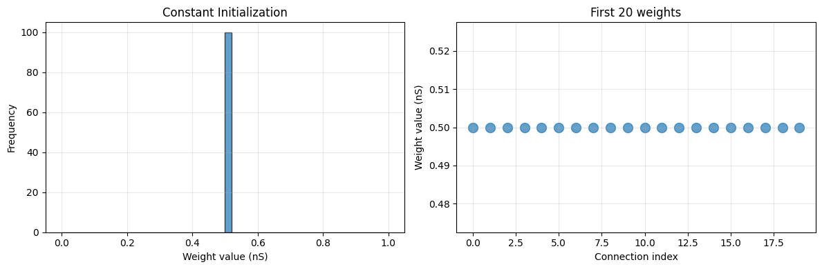
../_images/cbd3d834351d239aa3176aec679e43d69f9f0f41c8b627fcfdde100a5fa8f3e3.png

⚠️ Note: Constant initialization breaks symmetry and is rarely used for weights!

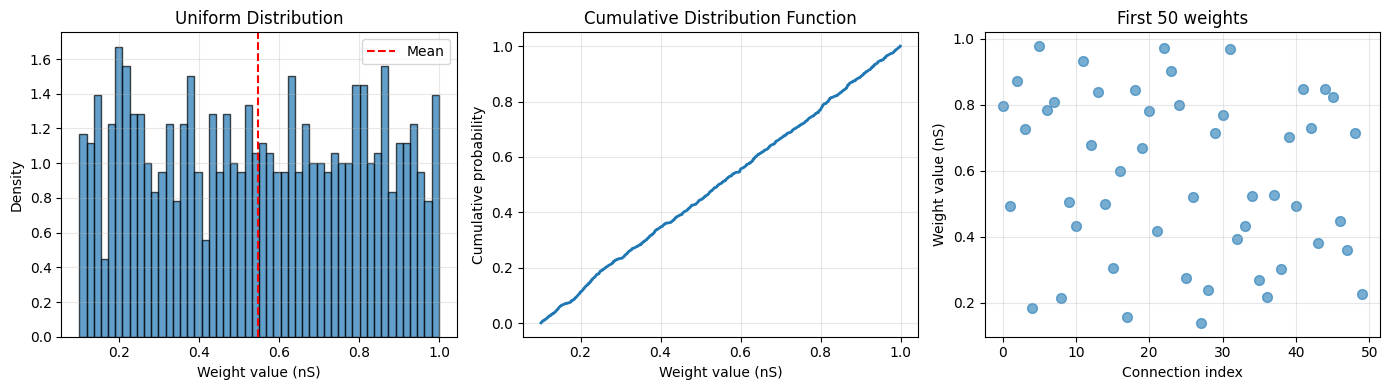
2.2 Uniform Distribution#

Uniform distribution generates weights with equal probability across a range [low, high). This is better than constant initialization as it breaks symmetry.

Use cases:

Simple baseline initialization
When you want bounded weights
Embedding layers

# Create uniform initializer
uniform_init = init.Uniform(low=0.1 * u.nS, high=1.0 * u.nS)

# Generate weights
weights = uniform_init(1000, rng=rng)

print(f"Uniform initialization:")
print(f"  Shape: {weights.shape}")
print(f"  Min: {weights.min():.3f}")
print(f"  Max: {weights.max():.3f}")
print(f"  Mean: {weights.mean():.3f}")
print(f"  Std: {weights.std():.3f}")

# Visualize
fig, axes = plt.subplots(1, 3, figsize=(14, 4))

# Histogram
axes[0].hist(weights.mantissa, bins=50, alpha=0.7, edgecolor='black', density=True)
axes[0].axvline(weights.mean().mantissa, color='red', linestyle='--', label='Mean')
axes[0].set_xlabel(f'Weight value ({weights.unit})')
axes[0].set_ylabel('Density')
axes[0].set_title('Uniform Distribution')
axes[0].legend()
axes[0].grid(alpha=0.3)

# CDF
sorted_weights = np.sort(weights.mantissa)
cdf = np.arange(1, len(sorted_weights) + 1) / len(sorted_weights)
axes[1].plot(sorted_weights, cdf, linewidth=2)
axes[1].set_xlabel(f'Weight value ({weights.unit})')
axes[1].set_ylabel('Cumulative probability')
axes[1].set_title('Cumulative Distribution Function')
axes[1].grid(alpha=0.3)

# Sample weights
axes[2].scatter(range(50), weights[:50].mantissa, s=50, alpha=0.6)
axes[2].set_xlabel('Connection index')
axes[2].set_ylabel(f'Weight value ({weights.unit})')
axes[2].set_title('First 50 weights')
axes[2].grid(alpha=0.3)

plt.tight_layout()
plt.show()

Uniform initialization:
  Shape: (1000,)
  Min: 0.101 * nsiemens
  Max: 0.999 * nsiemens
  Mean: 0.547 * nsiemens
  Std: 0.262 * nsiemens

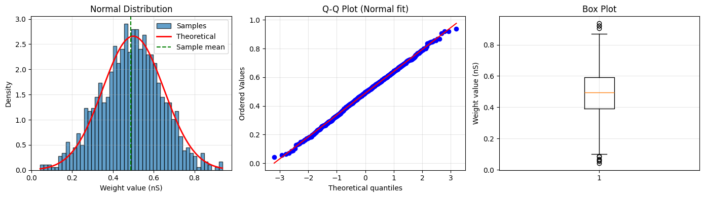
../_images/cf82ccf62f08c3703f04ff810f823d74a6793da055b52ee3581d75494d881083.png

2.3 Normal (Gaussian) Distribution#

Normal distribution is one of the most common initialization strategies. It generates weights from a Gaussian with specified mean and standard deviation.

Use cases:

General purpose initialization
When combined with variance scaling (covered in Tutorial 2)
Biological plausibility (many neural properties are normally distributed)

# Create normal initializer
normal_init = init.Normal(mean=0.5 * u.nS, std=0.15 * u.nS)

# Generate weights
weights = normal_init(1000, rng=rng)

print(f"Normal initialization:")
print(f"  Shape: {weights.shape}")
print(f"  Min: {weights.min():.3f}")
print(f"  Max: {weights.max():.3f}")
print(f"  Mean: {weights.mean():.3f}")
print(f"  Std: {weights.std():.3f}")

# Visualize
fig, axes = plt.subplots(1, 3, figsize=(14, 4))

# Histogram with theoretical curve
counts, bins, _ = axes[0].hist(weights.mantissa,
                               bins=50,
                               alpha=0.7,
                               edgecolor='black',
                               density=True,
                               label='Samples')
x = np.linspace(weights.min().mantissa, weights.max().mantissa, 100)
theoretical = (1 / (0.15 * np.sqrt(2 * np.pi))) * np.exp(-0.5 * ((x - 0.5) / 0.15) ** 2)
axes[0].plot(x, theoretical, 'r-', linewidth=2, label='Theoretical')
axes[0].axvline(weights.mean().mantissa, color='green', linestyle='--', label='Sample mean')
axes[0].set_xlabel(f'Weight value ({weights.unit})')
axes[0].set_ylabel('Density')
axes[0].set_title('Normal Distribution')
axes[0].legend()
axes[0].grid(alpha=0.3)

# Q-Q plot
from scipy import stats

stats.probplot(weights.mantissa, dist="norm", plot=axes[1])
axes[1].set_title('Q-Q Plot (Normal fit)')
axes[1].grid(alpha=0.3)

# Box plot
axes[2].boxplot(weights.mantissa, vert=True)
axes[2].set_ylabel(f'Weight value ({weights.unit})')
axes[2].set_title('Box Plot')
axes[2].grid(alpha=0.3)

plt.tight_layout()
plt.show()

Normal initialization:
  Shape: (1000,)
  Min: 0.043 * nsiemens
  Max: 0.937 * nsiemens
  Mean: 0.488 * nsiemens
  Std: 0.152 * nsiemens

../_images/84cb70c5eef3eca10e6a2b5675da4d27e87151b38b56a50745afdd90bc78a52c.png

Comparing Basic Distributions#

# Compare the three basic distributions
n_samples = 5000

constant_weights = init.Constant(0.5 * u.nS)(n_samples)
uniform_weights = init.Uniform(0.1 * u.nS, 0.9 * u.nS)(n_samples, rng=rng)
normal_weights = init.Normal(0.5 * u.nS, 0.15 * u.nS)(n_samples, rng=rng)

fig, axes = plt.subplots(1, 3, figsize=(15, 4))

for ax, weights, title in zip(axes,
                              [constant_weights, uniform_weights, normal_weights],
                              ['Constant', 'Uniform', 'Normal']):
    ax.hist(weights.mantissa, bins=50, alpha=0.7, edgecolor='black', density=True)
    ax.axvline(weights.mean().mantissa, color='red', linestyle='--',
               label=f'Mean: {weights.mean():.3f}')
    ax.set_xlabel(f'Weight value ({weights.unit})')
    ax.set_ylabel('Density')
    ax.set_title(title)
    ax.legend()
    ax.grid(alpha=0.3)

plt.tight_layout()
plt.show()

# Statistics comparison
print("\nComparison of Basic Distributions:")
print("-" * 60)
print(f"{'Distribution':<15} {'Mean':<15} {'Std':<15} {'Range'}")
print("-" * 60)
print(f"{'Constant':<15} {constant_weights.mean()!s:<15} {constant_weights.std()!s:<15} "
      f"[{constant_weights.min():.2f}, {constant_weights.max():.2f}]")
print(f"{'Uniform':<15} {uniform_weights.mean()!s:<15} {uniform_weights.std()!s:<15} "
      f"[{uniform_weights.min():.2f}, {uniform_weights.max():.2f}]")
print(f"{'Normal':<15} {normal_weights.mean()!s:<15} {normal_weights.std()!s:<15} "
      f"[{normal_weights.min():.2f}, {normal_weights.max():.2f}]")

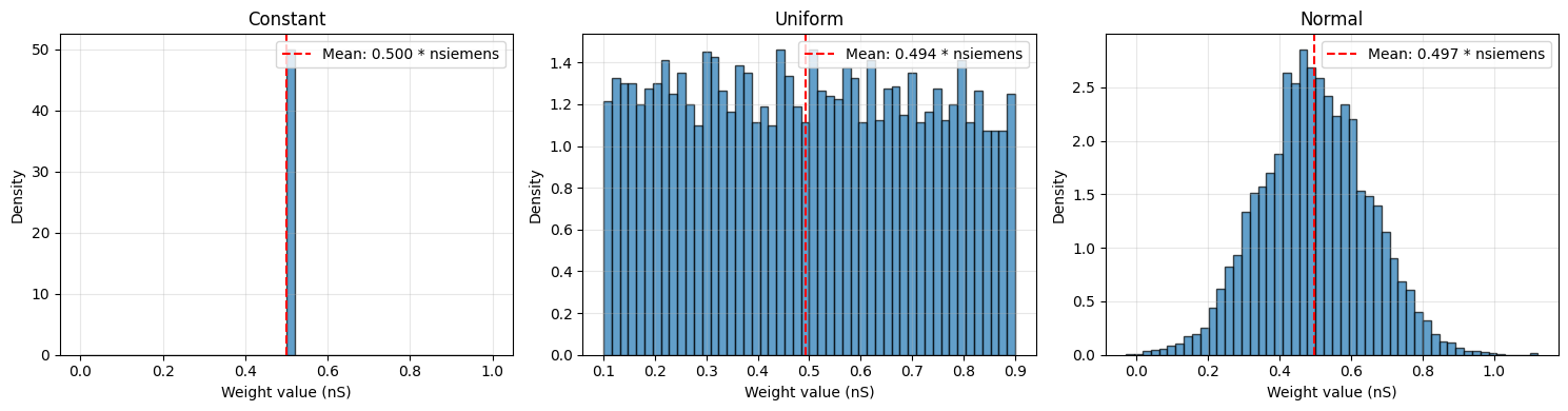
../_images/b243ebb543562c1d15085d7d564e004562e298af759bb4d731a1fbebca1a3e2e.png

Comparison of Basic Distributions:
------------------------------------------------------------
Distribution    Mean            Std             Range
------------------------------------------------------------
Constant        0.5 * nsiemens  0. * nsiemens   [0.50 * nsiemens, 0.50 * nsiemens]
Uniform         0.49354032 * nsiemens 0.22933985 * nsiemens [0.10 * nsiemens, 0.90 * nsiemens]
Normal          0.49672538 * nsiemens 0.15104583 * nsiemens [-0.03 * nsiemens, 1.12 * nsiemens]

3. Statistical Distributions#

BrainTools provides several advanced statistical distributions that are useful for specific scenarios in neuroscience and machine learning.

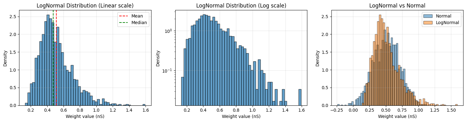
3.1 LogNormal Distribution#

LogNormal distribution generates positive values with a long tail. It’s particularly useful for:

Synaptic weights: Many biological measurements are log-normally distributed
Positive-only values: When weights must be positive
Multiplicative processes: Natural for growth/decay processes

# Create log-normal initializer
# Note: mean and std are in LINEAR space (not log-space)
lognormal_init = init.LogNormal(mean=0.5 * u.nS, std=0.2 * u.nS)

# Generate weights
weights = lognormal_init(2000, rng=rng)

print(f"LogNormal initialization:")
print(f"  Mean: {weights.mean():.3f}")
print(f"  Std: {weights.std():.3f}")
print(f"  Median: {u.math.median(weights):.3f}")
print(f"  Skewness: {((weights.mantissa - weights.mean().mantissa) ** 3).mean() / weights.std().mantissa ** 3:.3f}")

# Visualize
fig, axes = plt.subplots(1, 3, figsize=(15, 4))

# Histogram (linear scale)
axes[0].hist(weights.mantissa, bins=50, alpha=0.7, edgecolor='black', density=True)
axes[0].axvline(weights.mean().mantissa, color='red', linestyle='--', label='Mean')
axes[0].axvline(u.math.median(weights).mantissa, color='green', linestyle='--', label='Median')
axes[0].set_xlabel(f'Weight value ({weights.unit})')
axes[0].set_ylabel('Density')
axes[0].set_title('LogNormal Distribution (Linear scale)')
axes[0].legend()
axes[0].grid(alpha=0.3)

# Histogram (log scale)
axes[1].hist(weights.mantissa, bins=50, alpha=0.7, edgecolor='black', density=True)
axes[1].set_xlabel(f'Weight value ({weights.unit})')
axes[1].set_ylabel('Density')
axes[1].set_title('LogNormal Distribution (Log scale)')
axes[1].set_yscale('log')
axes[1].grid(alpha=0.3)

# Compare with Normal
normal_weights = init.Normal(0.5 * u.nS, 0.2 * u.nS)(2000, rng=rng)
axes[2].hist(normal_weights.mantissa, bins=50, alpha=0.5,
             label='Normal', edgecolor='black', density=True)
axes[2].hist(weights.mantissa, bins=50, alpha=0.5,
             label='LogNormal', edgecolor='black', density=True)
axes[2].set_xlabel(f'Weight value ({weights.unit})')
axes[2].set_ylabel('Density')
axes[2].set_title('LogNormal vs Normal')
axes[2].legend()
axes[2].grid(alpha=0.3)

plt.tight_layout()
plt.show()

LogNormal initialization:
  Mean: 0.511 * nsiemens
  Std: 0.202 * nsiemens
  Median: 0.473 * nsiemens
  Skewness: 1.106

../_images/08f683120f20818623bfd9ac548cdf15d828ba9432d6d39992342d9a43590b09.png

3.2 Gamma Distribution#

Gamma distribution is useful for positive-valued weights with controllable shape and scale.

Use cases:

Modeling waiting times or intervals
Positive weights with specific skewness
Rate parameters in Poisson processes

# Create gamma initializers with different parameters
gamma_init_1 = init.Gamma(shape=2.0, scale=0.25 * u.nS)
gamma_init_2 = init.Gamma(shape=5.0, scale=0.1 * u.nS)
gamma_init_3 = init.Gamma(shape=10.0, scale=0.05 * u.nS)

# Generate weights
weights_1 = gamma_init_1(2000, rng=rng)
weights_2 = gamma_init_2(2000, rng=rng)
weights_3 = gamma_init_3(2000, rng=rng)

# Visualize
fig, axes = plt.subplots(1, 2, figsize=(12, 4))

# Overlay different gamma distributions
axes[0].hist(weights_1.mantissa, bins=50, alpha=0.5, label='shape=2.0, scale=0.25',
             density=True, edgecolor='black')
axes[0].hist(weights_2.mantissa, bins=50, alpha=0.5, label='shape=5.0, scale=0.1',
             density=True, edgecolor='black')
axes[0].hist(weights_3.mantissa, bins=50, alpha=0.5, label='shape=10.0, scale=0.05',
             density=True, edgecolor='black')
axes[0].set_xlabel(f'Weight value ({weights_1.unit})')
axes[0].set_ylabel('Density')
axes[0].set_title('Gamma Distribution with Different Parameters')
axes[0].legend()
axes[0].grid(alpha=0.3)

# Statistics comparison
distributions = ['shape=2.0', 'shape=5.0', 'shape=10.0']
means = [weights_1.mean().mantissa, weights_2.mean().mantissa, weights_3.mean().mantissa]
stds = [weights_1.std().mantissa, weights_2.std().mantissa, weights_3.std().mantissa]

x = np.arange(len(distributions))
width = 0.35
axes[1].bar(x - width / 2, means, width, label='Mean', alpha=0.7)
axes[1].bar(x + width / 2, stds, width, label='Std', alpha=0.7)
axes[1].set_ylabel(f'Value ({weights_1.unit})')
axes[1].set_title('Mean and Std for Different Gamma Parameters')
axes[1].set_xticks(x)
axes[1].set_xticklabels(distributions, rotation=15)
axes[1].legend()
axes[1].grid(alpha=0.3, axis='y')

plt.tight_layout()
plt.show()

print("\nGamma Distribution Properties:")
print("-" * 50)
for i, (name, w) in enumerate(zip(distributions, [weights_1, weights_2, weights_3])):
    print(f"{name}: mean={w.mean():.3f}, std={w.std():.3f}")

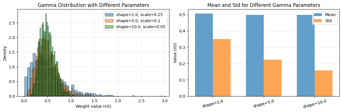
../_images/beb315d22f5191dad6750d8b0517186de446334b3dbd474ed9c88b3af66c369d.png

Gamma Distribution Properties:
--------------------------------------------------
shape=2.0: mean=0.507 * nsiemens, std=0.350 * nsiemens
shape=5.0: mean=0.498 * nsiemens, std=0.224 * nsiemens
shape=10.0: mean=0.499 * nsiemens, std=0.159 * nsiemens

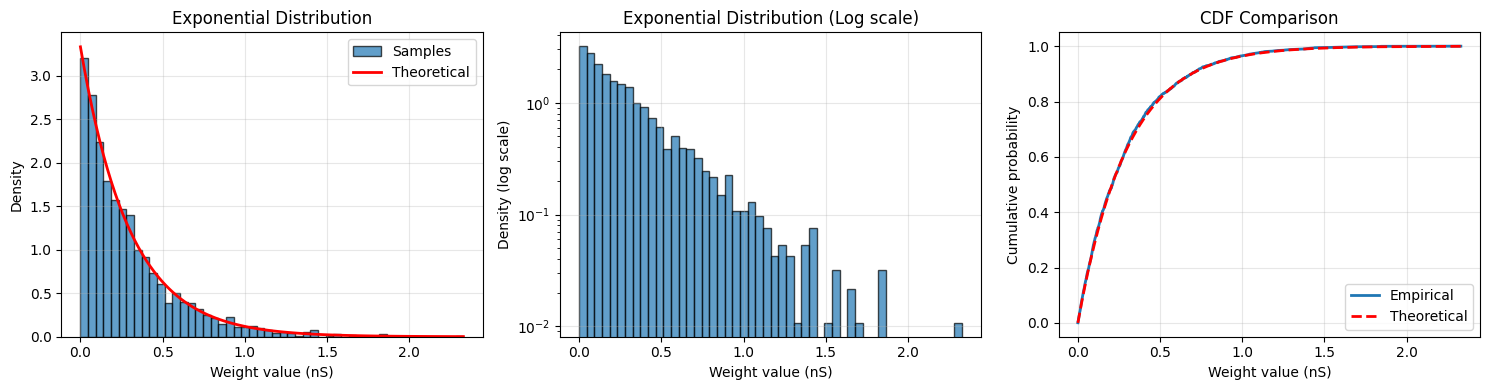
3.3 Exponential Distribution#

Exponential distribution models time between events in a Poisson process.

Use cases:

Modeling decay processes
Inter-spike intervals
Positive weights with maximum entropy for given mean

# Create exponential initializer
exponential_init = init.Exponential(scale=0.3 * u.nS)

# Generate weights
weights = exponential_init(2000, rng=rng)

print(f"Exponential initialization:")
print(f"  Mean: {weights.mean():.3f}")
print(f"  Std: {weights.std():.3f}")
print(f"  Theoretical mean: {0.3 * u.nS}")
print(f"  Theoretical std: {0.3 * u.nS}")

# Visualize
fig, axes = plt.subplots(1, 3, figsize=(15, 4))

# Histogram with theoretical curve
counts, bins, _ = axes[0].hist(weights.mantissa, bins=50, alpha=0.7,
                               edgecolor='black', density=True, label='Samples')
x = np.linspace(0, weights.max().mantissa, 100)
theoretical = (1 / 0.3) * np.exp(-x / 0.3)
axes[0].plot(x, theoretical, 'r-', linewidth=2, label='Theoretical')
axes[0].set_xlabel(f'Weight value ({weights.unit})')
axes[0].set_ylabel('Density')
axes[0].set_title('Exponential Distribution')
axes[0].legend()
axes[0].grid(alpha=0.3)

# Log scale histogram
axes[1].hist(weights.mantissa, bins=50, alpha=0.7, edgecolor='black', density=True)
axes[1].set_xlabel(f'Weight value ({weights.unit})')
axes[1].set_ylabel('Density (log scale)')
axes[1].set_title('Exponential Distribution (Log scale)')
axes[1].set_yscale('log')
axes[1].grid(alpha=0.3)

# Cumulative distribution
sorted_weights = np.sort(weights.mantissa)
cdf = np.arange(1, len(sorted_weights) + 1) / len(sorted_weights)
theoretical_cdf = 1 - np.exp(-sorted_weights / 0.3)
axes[2].plot(sorted_weights, cdf, label='Empirical', linewidth=2)
axes[2].plot(sorted_weights, theoretical_cdf, 'r--', label='Theoretical', linewidth=2)
axes[2].set_xlabel(f'Weight value ({weights.unit})')
axes[2].set_ylabel('Cumulative probability')
axes[2].set_title('CDF Comparison')
axes[2].legend()
axes[2].grid(alpha=0.3)

plt.tight_layout()
plt.show()

Exponential initialization:
  Mean: 0.295 * nsiemens
  Std: 0.294 * nsiemens
  Theoretical mean: 0.3 * nsiemens
  Theoretical std: 0.3 * nsiemens

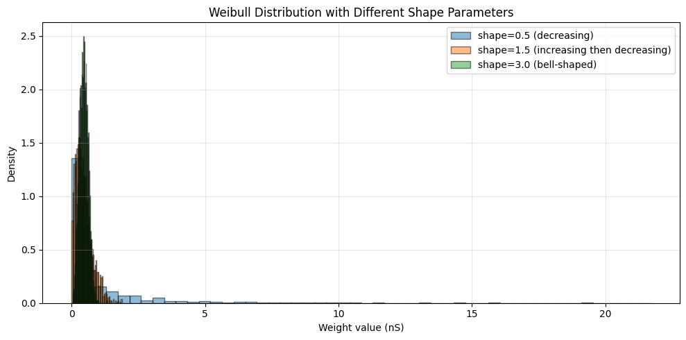
../_images/9d3d62634f1f9862f323dd3db00534a1829471bc47642d1e50cc84cd07d451e5.png

3.4 Weibull Distribution#

Weibull distribution is a generalization of the exponential distribution with an additional shape parameter.

Use cases:

Modeling failure rates or lifetimes
Flexible shape for positive-valued weights
When you need more control than exponential

# Create Weibull initializers with different shapes
weibull_init_1 = init.Weibull(shape=0.5, scale=0.5 * u.nS)
weibull_init_2 = init.Weibull(shape=1.5, scale=0.5 * u.nS)
weibull_init_3 = init.Weibull(shape=3.0, scale=0.5 * u.nS)

# Generate weights
weights_1 = weibull_init_1(2000, rng=rng)
weights_2 = weibull_init_2(2000, rng=rng)
weights_3 = weibull_init_3(2000, rng=rng)

# Visualize
fig, ax = plt.subplots(1, 1, figsize=(10, 5))

ax.hist(weights_1.mantissa, bins=50, alpha=0.5, label='shape=0.5 (decreasing)',
        density=True, edgecolor='black')
ax.hist(weights_2.mantissa, bins=50, alpha=0.5, label='shape=1.5 (increasing then decreasing)',
        density=True, edgecolor='black')
ax.hist(weights_3.mantissa, bins=50, alpha=0.5, label='shape=3.0 (bell-shaped)',
        density=True, edgecolor='black')
ax.set_xlabel(f'Weight value ({weights_1.unit})')
ax.set_ylabel('Density')
ax.set_title('Weibull Distribution with Different Shape Parameters')
ax.legend()
ax.grid(alpha=0.3)

plt.tight_layout()
plt.show()

print("\nWeibull Distribution Shape Effects:")
print("-" * 60)
print("shape < 1: High failure rate early, then decreasing")
print("shape = 1: Constant failure rate (exponential distribution)")
print("shape > 1: Failure rate increases over time")

../_images/e411443b5e420e9a67b794deb70a4461f1d571e4dc722d2e1b4de0f0306bd70a.png

Weibull Distribution Shape Effects:
------------------------------------------------------------
shape < 1: High failure rate early, then decreasing
shape = 1: Constant failure rate (exponential distribution)
shape > 1: Failure rate increases over time

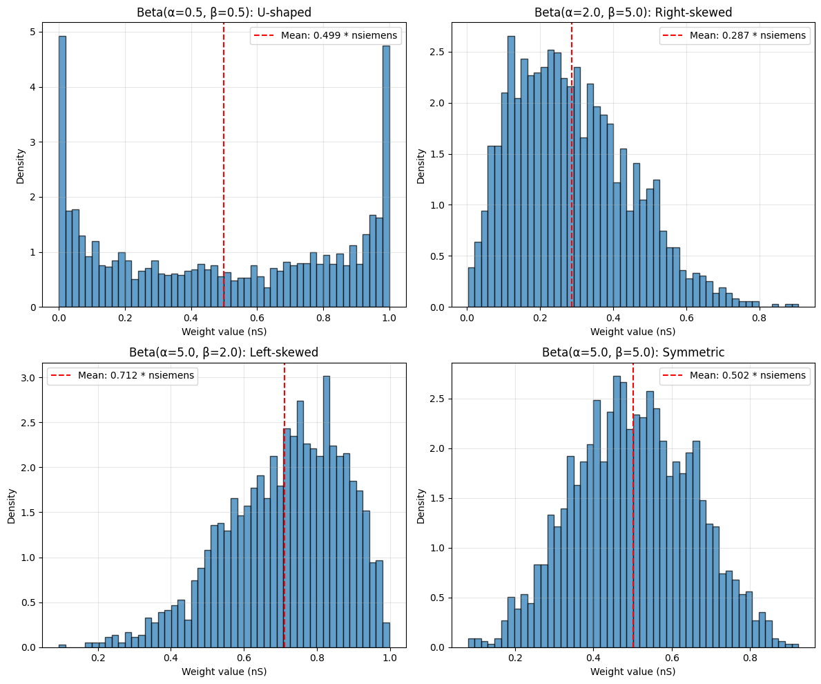
3.5 Beta Distribution#

Beta distribution generates values in a bounded range [0, 1] (or rescaled to [low, high]). It’s extremely flexible with two shape parameters.

Use cases:

Bounded weights (e.g., probabilities, proportions)
Flexible shapes (uniform, U-shaped, bell-shaped, J-shaped)
Modeling ratios or percentages

# Create Beta initializers with different parameters
beta_init_1 = init.Beta(alpha=0.5, beta=0.5, low=0.0 * u.nS, high=1.0 * u.nS)  # U-shaped
beta_init_2 = init.Beta(alpha=2.0, beta=5.0, low=0.0 * u.nS, high=1.0 * u.nS)  # Right-skewed
beta_init_3 = init.Beta(alpha=5.0, beta=2.0, low=0.0 * u.nS, high=1.0 * u.nS)  # Left-skewed
beta_init_4 = init.Beta(alpha=5.0, beta=5.0, low=0.0 * u.nS, high=1.0 * u.nS)  # Symmetric

# Generate weights
weights_1 = beta_init_1(2000, rng=rng)
weights_2 = beta_init_2(2000, rng=rng)
weights_3 = beta_init_3(2000, rng=rng)
weights_4 = beta_init_4(2000, rng=rng)

# Visualize
fig, axes = plt.subplots(2, 2, figsize=(12, 10))
axes = axes.flatten()

params = [(0.5, 0.5, 'U-shaped'), (2.0, 5.0, 'Right-skewed'),
          (5.0, 2.0, 'Left-skewed'), (5.0, 5.0, 'Symmetric')]
weights_list = [weights_1, weights_2, weights_3, weights_4]

for ax, (alpha, beta, name), weights in zip(axes, params, weights_list):
    ax.hist(weights.mantissa, bins=50, alpha=0.7, edgecolor='black', density=True)
    ax.axvline(weights.mean().mantissa, color='red', linestyle='--',
               label=f'Mean: {weights.mean():.3f}')
    ax.set_xlabel(f'Weight value ({weights.unit})')
    ax.set_ylabel('Density')
    ax.set_title(f'Beta(α={alpha}, β={beta}): {name}')
    ax.legend()
    ax.grid(alpha=0.3)

plt.tight_layout()
plt.show()

print("\nBeta Distribution Shape Guide:")
print("-" * 60)
print("α < 1, β < 1: U-shaped (high at boundaries)")
print("α < 1, β ≥ 1: J-shaped (decreasing from 0)")
print("α ≥ 1, β < 1: Reverse J-shaped (increasing to 1)")
print("α = β: Symmetric around 0.5")
print("α > β: Left-skewed (peak towards 1)")
print("α < β: Right-skewed (peak towards 0)")

../_images/f50b6884267d4082c02958b6be8437ee75d194ed9ae63b53bb20423e1ff3c56d.png

Beta Distribution Shape Guide:
------------------------------------------------------------
α < 1, β < 1: U-shaped (high at boundaries)
α < 1, β ≥ 1: J-shaped (decreasing from 0)
α ≥ 1, β < 1: Reverse J-shaped (increasing to 1)
α = β: Symmetric around 0.5
α > β: Left-skewed (peak towards 1)
α < β: Right-skewed (peak towards 0)

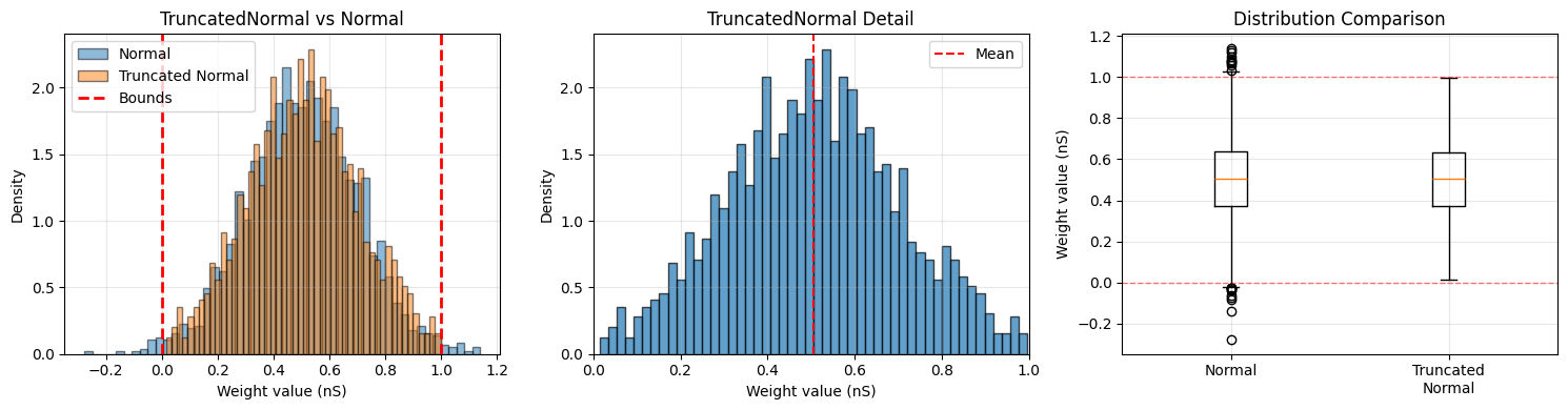
4. TruncatedNormal Distribution#

TruncatedNormal is a normal distribution cut off at specified bounds. This is particularly useful when you want Gaussian properties but need to ensure weights stay within a specific range.

Use cases:

Bounded weights with Gaussian-like properties
Preventing extreme outliers
Physical constraints (e.g., conductances must be positive)

# Create truncated normal initializer
truncated_init = init.TruncatedNormal(
    mean=0.5 * u.nS,
    std=0.2 * u.nS,
    low=0.0 * u.nS,
    high=1.0 * u.nS
)

# Generate weights
truncated_weights = truncated_init(2000, rng=rng)

# Compare with regular normal
normal_init = init.Normal(mean=0.5 * u.nS, std=0.2 * u.nS)
normal_weights = normal_init(2000, rng=rng)

print(f"TruncatedNormal initialization:")
print(f"  Mean: {truncated_weights.mean():.3f}")
print(f"  Std: {truncated_weights.std():.3f}")
print(f"  Min: {truncated_weights.min():.3f}")
print(f"  Max: {truncated_weights.max():.3f}")
print(f"\nRegular Normal (for comparison):")
print(f"  Mean: {normal_weights.mean():.3f}")
print(f"  Std: {normal_weights.std():.3f}")
print(f"  Min: {normal_weights.min():.3f}")
print(f"  Max: {normal_weights.max():.3f}")
print(f"  Values outside [0, 1]: {np.sum((normal_weights.mantissa < 0) | (normal_weights.mantissa > 1))}")

# Visualize
fig, axes = plt.subplots(1, 3, figsize=(15, 4))

# Comparison histogram
axes[0].hist(normal_weights.mantissa, bins=50, alpha=0.5, label='Normal',
             density=True, edgecolor='black')
axes[0].hist(truncated_weights.mantissa, bins=50, alpha=0.5, label='Truncated Normal',
             density=True, edgecolor='black')
axes[0].axvline(0.0, color='red', linestyle='--', linewidth=2, label='Bounds')
axes[0].axvline(1.0, color='red', linestyle='--', linewidth=2)
axes[0].set_xlabel(f'Weight value ({truncated_weights.unit})')
axes[0].set_ylabel('Density')
axes[0].set_title('TruncatedNormal vs Normal')
axes[0].legend()
axes[0].grid(alpha=0.3)

# Zoom in on truncated region
axes[1].hist(truncated_weights.mantissa, bins=50, alpha=0.7, edgecolor='black', density=True)
axes[1].axvline(truncated_weights.mean().mantissa, color='red', linestyle='--', label='Mean')
axes[1].set_xlabel(f'Weight value ({truncated_weights.unit})')
axes[1].set_ylabel('Density')
axes[1].set_title('TruncatedNormal Detail')
axes[1].set_xlim([0, 1])
axes[1].legend()
axes[1].grid(alpha=0.3)

# Box plot comparison
axes[2].boxplot([normal_weights.mantissa, truncated_weights.mantissa],
                tick_labels=['Normal', 'Truncated\nNormal'])
axes[2].axhline(0.0, color='red', linestyle='--', linewidth=1, alpha=0.5)
axes[2].axhline(1.0, color='red', linestyle='--', linewidth=1, alpha=0.5)
axes[2].set_ylabel(f'Weight value ({truncated_weights.unit})')
axes[2].set_title('Distribution Comparison')
axes[2].grid(alpha=0.3)

plt.tight_layout()
plt.show()

TruncatedNormal initialization:
  Mean: 0.505 * nsiemens
  Std: 0.196 * nsiemens
  Min: 0.014 * nsiemens
  Max: 0.997 * nsiemens

Regular Normal (for comparison):
  Mean: 0.503 * nsiemens
  Std: 0.199 * nsiemens
  Min: -0.278 * nsiemens
  Max: 1.139 * nsiemens
  Values outside [0, 1]: 30

../_images/68fce09d1569200043a2def571adfcce9e3508b01ccb268e5d890b9f0444c9c9.png

Effect of Truncation Bounds#

# Compare different truncation bounds
truncated_tight = init.TruncatedNormal(0.5 * u.nS, 0.2 * u.nS,
                                       0.3 * u.nS, 0.7 * u.nS)(2000, rng=rng)
truncated_medium = init.TruncatedNormal(0.5 * u.nS, 0.2 * u.nS,
                                        0.1 * u.nS, 0.9 * u.nS)(2000, rng=rng)
truncated_wide = init.TruncatedNormal(0.5 * u.nS, 0.2 * u.nS,
                                      -0.1 * u.nS, 1.1 * u.nS)(2000, rng=rng)

fig, ax = plt.subplots(1, 1, figsize=(10, 5))

ax.hist(truncated_tight.mantissa, bins=50, alpha=0.5,
        label='Tight [0.3, 0.7]', density=True, edgecolor='black')
ax.hist(truncated_medium.mantissa, bins=50, alpha=0.5,
        label='Medium [0.1, 0.9]', density=True, edgecolor='black')
ax.hist(truncated_wide.mantissa, bins=50, alpha=0.5,
        label='Wide [-0.1, 1.1]', density=True, edgecolor='black')
ax.set_xlabel(f'Weight value ({truncated_tight.unit})')
ax.set_ylabel('Density')
ax.set_title('Effect of Truncation Bounds')
ax.legend()
ax.grid(alpha=0.3)

plt.tight_layout()
plt.show()

print("\nEffect of Truncation Bounds:")
print("-" * 60)
print(f"Tight [0.3, 0.7]:   mean={truncated_tight.mean():.3f}, std={truncated_tight.std():.3f}")
print(f"Medium [0.1, 0.9]:  mean={truncated_medium.mean():.3f}, std={truncated_medium.std():.3f}")
print(f"Wide [-0.1, 1.1]:   mean={truncated_wide.mean():.3f}, std={truncated_wide.std():.3f}")
print("\nNote: Tighter bounds reduce variance and shift the mean toward the center of the truncation range.")

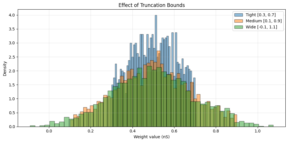
../_images/1cca23023288edda22c3999643151a4a7f4fac4b30b16a6e604f5a64d52240a7.png

Effect of Truncation Bounds:
------------------------------------------------------------
Tight [0.3, 0.7]:   mean=0.503 * nsiemens, std=0.105 * nsiemens
Medium [0.1, 0.9]:  mean=0.498 * nsiemens, std=0.175 * nsiemens
Wide [-0.1, 1.1]:   mean=0.497 * nsiemens, std=0.196 * nsiemens

Note: Tighter bounds reduce variance and shift the mean toward the center of the truncation range.

5. Practical Examples with BrainUnit Quantities#

Let’s explore how to use these initializers in realistic neuroscience scenarios with physical units.

Example 1: Excitatory and Inhibitory Synaptic Conductances#

# Excitatory synapses: typically 0.5-3.0 nS
excitatory_init = init.TruncatedNormal(
    mean=1.5 * u.nS,
    std=0.5 * u.nS,
    low=0.5 * u.nS,
    high=3.0 * u.nS
)

# Inhibitory synapses: typically 2-10 nS (stronger)
inhibitory_init = init.LogNormal(
    mean=5.0 * u.nS,
    std=2.0 * u.nS
)

# Generate synaptic weights
n_excitatory = 800
n_inhibitory = 200

exc_weights = excitatory_init(n_excitatory, rng=rng)
inh_weights = inhibitory_init(n_inhibitory, rng=rng)

# Visualize
fig, axes = plt.subplots(1, 2, figsize=(12, 4))

axes[0].hist(exc_weights.mantissa, bins=40, alpha=0.7, label='Excitatory',
             edgecolor='black', color='red')
axes[0].hist(inh_weights.mantissa, bins=40, alpha=0.7, label='Inhibitory',
             edgecolor='black', color='blue')
axes[0].set_xlabel(f'Conductance ({exc_weights.unit})')
axes[0].set_ylabel('Count')
axes[0].set_title('Excitatory vs Inhibitory Conductances')
axes[0].legend()
axes[0].grid(alpha=0.3)

# Create connection matrix visualization
all_weights = np.concatenate([exc_weights.mantissa, inh_weights.mantissa])
colors = ['red'] * n_excitatory + ['blue'] * n_inhibitory
axes[1].scatter(range(len(all_weights)), all_weights, c=colors, alpha=0.5, s=20)
axes[1].axhline(exc_weights.mean().mantissa, color='red', linestyle='--',
                label=f'Exc mean: {exc_weights.mean():.2f}')
axes[1].axhline(inh_weights.mean().mantissa, color='blue', linestyle='--',
                label=f'Inh mean: {inh_weights.mean():.2f}')
axes[1].set_xlabel('Synapse index')
axes[1].set_ylabel(f'Conductance ({exc_weights.unit})')
axes[1].set_title('Synaptic Weight Distribution')
axes[1].legend()
axes[1].grid(alpha=0.3)

plt.tight_layout()
plt.show()

print(f"Excitatory synapses (n={n_excitatory}):")
print(f"  Mean: {exc_weights.mean():.3f}")
print(f"  Std: {exc_weights.std():.3f}")
print(f"  Range: [{exc_weights.min():.2f}, {exc_weights.max():.2f}]")
print(f"\nInhibitory synapses (n={n_inhibitory}):")
print(f"  Mean: {inh_weights.mean():.3f}")
print(f"  Std: {inh_weights.std():.3f}")
print(f"  Range: [{inh_weights.min():.2f}, {inh_weights.max():.2f}]")

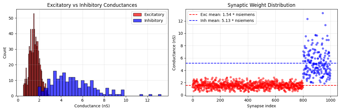
../_images/421ba49a4dc603c4610fcd0e66def3ac45708ea60b81568f44be95f30706608f.png

Excitatory synapses (n=800):
  Mean: 1.539 * nsiemens
  Std: 0.470 * nsiemens
  Range: [0.50 * nsiemens, 2.87 * nsiemens]

Inhibitory synapses (n=200):
  Mean: 5.132 * nsiemens
  Std: 2.015 * nsiemens
  Range: [1.86 * nsiemens, 13.26 * nsiemens]

Example 2: Spike Rate Parameters#

# Firing rates typically follow Gamma or LogNormal distributions
# Using Gamma for baseline firing rates
rate_init = init.Gamma(shape=3.0, scale=5.0 * u.Hz)

# Generate firing rates for a population
n_neurons = 500
firing_rates = rate_init(n_neurons, rng=rng)

# Visualize
fig, axes = plt.subplots(1, 3, figsize=(15, 4))

# Histogram
axes[0].hist(firing_rates.mantissa, bins=40, alpha=0.7, edgecolor='black')
axes[0].axvline(firing_rates.mean().mantissa, color='red', linestyle='--',
                label=f'Mean: {firing_rates.mean():.1f}')
axes[0].set_xlabel(f'Firing rate ({firing_rates.unit})')
axes[0].set_ylabel('Count')
axes[0].set_title('Population Firing Rates')
axes[0].legend()
axes[0].grid(alpha=0.3)

# Spatial arrangement
neuron_positions = np.arange(n_neurons)
colors = firing_rates.mantissa
scatter = axes[1].scatter(neuron_positions, firing_rates.mantissa,
                          c=colors, cmap='viridis', s=20, alpha=0.6)
axes[1].set_xlabel('Neuron index')
axes[1].set_ylabel(f'Firing rate ({firing_rates.unit})')
axes[1].set_title('Spatial Distribution of Firing Rates')
plt.colorbar(scatter, ax=axes[1], label=f'Rate ({firing_rates.unit})')
axes[1].grid(alpha=0.3)

# Categorize neurons by activity level
low_rate = firing_rates.mantissa < 10
medium_rate = (firing_rates.mantissa >= 10) & (firing_rates.mantissa < 20)
high_rate = firing_rates.mantissa >= 20

categories = ['Low\n(<10 Hz)', 'Medium\n(10-20 Hz)', 'High\n(≥20 Hz)']
counts = [np.sum(low_rate), np.sum(medium_rate), np.sum(high_rate)]
axes[2].bar(categories, counts, alpha=0.7, edgecolor='black')
axes[2].set_ylabel('Number of neurons')
axes[2].set_title('Activity Level Distribution')
axes[2].grid(alpha=0.3, axis='y')

plt.tight_layout()
plt.show()

print(f"Firing rate statistics:")
print(f"  Mean: {firing_rates.mean():.2f}")
print(f"  Median: {u.math.median(firing_rates):.2f}")
print(f"  Std: {firing_rates.std():.2f}")
print(f"  Range: [{firing_rates.min():.1f}, {firing_rates.max():.1f}]")
print(f"\nActivity categories:")
print(f"  Low rate: {np.sum(low_rate)} neurons ({100 * np.sum(low_rate) / n_neurons:.1f}%)")
print(f"  Medium rate: {np.sum(medium_rate)} neurons ({100 * np.sum(medium_rate) / n_neurons:.1f}%)")
print(f"  High rate: {np.sum(high_rate)} neurons ({100 * np.sum(high_rate) / n_neurons:.1f}%)")

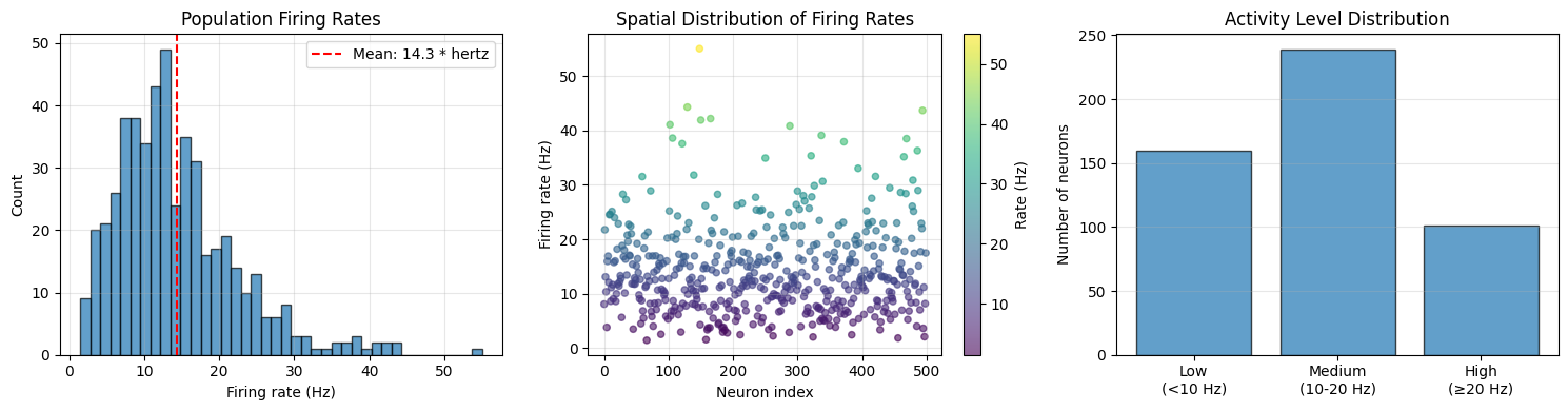
../_images/73d1ae0da0cdb2120bb49b4aa0717d96b54328b845dbfec1bda5a7da428365df.png

Firing rate statistics:
  Mean: 14.31 * hertz
  Median: 12.78 * hertz
  Std: 8.10 * hertz
  Range: [1.5 * hertz, 55.0 * hertz]

Activity categories:
  Low rate: 160 neurons (32.0%)
  Medium rate: 239 neurons (47.8%)
  High rate: 101 neurons (20.2%)

Example 3: Delay Times with Exponential Distribution#

# Synaptic delays often follow exponential distribution
delay_init = init.Exponential(scale=2.0 * u.ms)

# Generate axonal delays
n_connections = 1000
delays = delay_init(n_connections, rng=rng)

# Add a minimum delay (refractory period)
min_delay = 0.5 * u.ms
delays = delays + min_delay

# Visualize
fig, axes = plt.subplots(1, 2, figsize=(12, 4))

# Histogram
axes[0].hist(delays.mantissa, bins=50, alpha=0.7, edgecolor='black', density=True)
axes[0].axvline(delays.mean().mantissa, color='red', linestyle='--',
                label=f'Mean: {delays.mean():.2f}')
axes[0].set_xlabel(f'Delay ({delays.unit})')
axes[0].set_ylabel('Density')
axes[0].set_title('Synaptic Delay Distribution')
axes[0].legend()
axes[0].grid(alpha=0.3)

# Cumulative distribution
sorted_delays = np.sort(delays.mantissa)
cdf = np.arange(1, len(sorted_delays) + 1) / len(sorted_delays)
axes[1].plot(sorted_delays, cdf, linewidth=2)
axes[1].axhline(0.5, color='red', linestyle='--', alpha=0.5)
axes[1].axvline(u.math.median(delays).mantissa,
                color='red', linestyle='--',
                label=f'Median: {u.math.median(delays):.2f}')
axes[1].set_xlabel(f'Delay ({delays.unit})')
axes[1].set_ylabel('Cumulative probability')
axes[1].set_title('Cumulative Distribution')
axes[1].legend()
axes[1].grid(alpha=0.3)

plt.tight_layout()
plt.show()

print(f"Delay statistics:")
print(f"  Mean: {delays.mean():.2f}")
print(f"  Median: {u.math.median(delays):.2f}")
print(f"  Std: {delays.std():.2f}")
print(f"  Range: [{delays.min():.2f}, {delays.max():.2f}]")
print(f"  Delays < 5 ms: {100 * np.sum(delays.mantissa < 5) / n_connections:.1f}%")

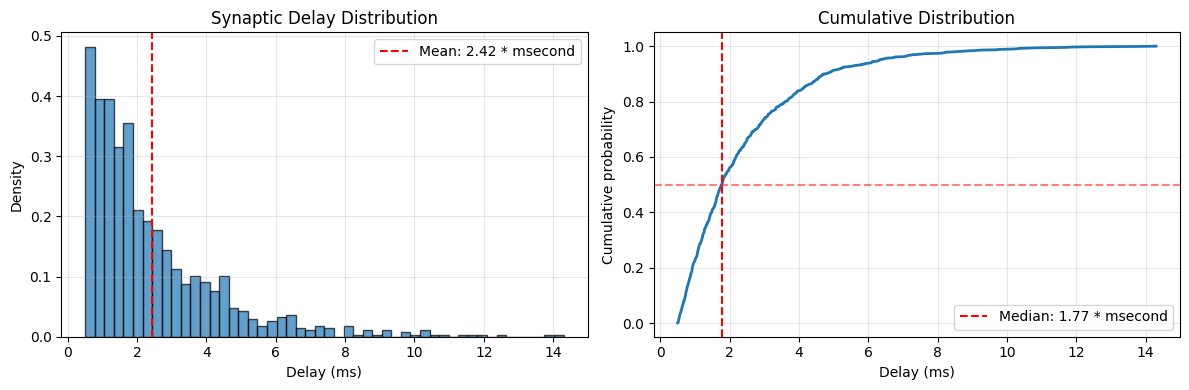
../_images/603c4d35a7ecf1c2e0bbbc3f8ebfe99a02e7ce84da5ad3fb3b4482ad38515a02.png

Delay statistics:
  Mean: 2.42 * msecond
  Median: 1.77 * msecond
  Std: 1.98 * msecond
  Range: [0.50 * msecond, 14.30 * msecond]
  Delays < 5 ms: 91.3%

6. When to Use Each Distribution Type#

This section provides practical guidance on choosing the right initialization distribution.

Decision Guide#

Distribution	When to Use	Advantages	Disadvantages
Constant	Biases only	Simple	Breaks symmetry for weights
Uniform	Baseline, embeddings	Equal probability, bounded	No special properties
Normal	General purpose	Well-studied, flexible	Unbounded, can produce outliers
LogNormal	Positive weights, biological	Positive, skewed, multiplicative	Complex parameter interpretation
Gamma	Rates, positive values	Flexible shape, positive	Two parameters to tune
Exponential	Delays, decay	Memoryless property, simple	Only one parameter (scale)
Weibull	Lifetimes, flexible positive	More flexible than exponential	Two parameters to tune
Beta	Bounded proportions	Very flexible, bounded	Two parameters to tune
TruncatedNormal	Bounded with Gaussian properties	Gaussian + bounds	More complex than Normal

Practical Recommendations

For Feed-forward Neural Networks:

Start with: Normal or Uniform
Better: Variance scaling methods (covered in Tutorial 2)
Best: Kaiming/Xavier initialization based on activation function

For Recurrent Neural Networks:

Start with: Normal with small std
Better: Orthogonal initialization (covered in Tutorial 2)
Best: Identity initialization + small Normal noise

For Biologically Realistic Models:

Conductances: LogNormal or TruncatedNormal
Firing rates: Gamma or LogNormal
Delays: Exponential + minimum delay
Probabilities: Beta distribution

For Reinforcement Learning:

Policy networks: Orthogonal for hidden layers, small Normal for output
Value networks: Xavier/Kaiming initialization

When You Need:

Strictly positive weights: LogNormal, Gamma, Exponential, Weibull
Bounded weights: Uniform, Beta, TruncatedNormal
Symmetric distribution: Normal, Uniform
Heavy tails: LogNormal, Weibull (shape < 1)
Light tails: TruncatedNormal, Beta, Weibull (shape > 3)

Comparison Example: All Distributions#

# Create a comprehensive comparison
n_samples = 5000

distributions = {
    'Constant': init.Constant(0.5 * u.nS),
    'Uniform': init.Uniform(0.2 * u.nS, 0.8 * u.nS),
    'Normal': init.Normal(0.5 * u.nS, 0.15 * u.nS),
    'LogNormal': init.LogNormal(0.5 * u.nS, 0.15 * u.nS),
    'Gamma': init.Gamma(5.0, 0.1 * u.nS),
    'Exponential': init.Exponential(0.5 * u.nS),
    'Weibull': init.Weibull(2.0, 0.5 * u.nS),
    'Beta': init.Beta(2.0, 5.0, 0.0 * u.nS, 1.0 * u.nS),
    'TruncatedNormal': init.TruncatedNormal(0.5 * u.nS, 0.15 * u.nS, 0.2 * u.nS, 0.8 * u.nS),
}

# Generate samples
samples = {}
for name, dist in distributions.items():
    if name == 'Constant':
        samples[name] = dist(n_samples)
    else:
        samples[name] = dist(n_samples, rng=rng)

# Visualize all distributions
fig, axes = plt.subplots(3, 3, figsize=(15, 12))
axes = axes.flatten()

for ax, (name, weights) in zip(axes, samples.items()):
    if name == 'Constant':
        ax.hist(weights.mantissa, bins=1, alpha=0.7, edgecolor='black')
    else:
        ax.hist(weights.mantissa, bins=50, alpha=0.7, edgecolor='black')
    ax.axvline(weights.mean().mantissa, color='red', linestyle='--',
               label=f'μ={weights.mean():.2f}')
    ax.set_xlabel(f'Value ({weights.unit})')
    ax.set_ylabel('Count')
    ax.set_title(name)
    ax.legend()
    ax.grid(alpha=0.3)

plt.tight_layout()
plt.show()

# Statistics table
print("\nStatistics Comparison:")
print("-" * 80)
print(f"{'Distribution':<20} {'Mean':<15} {'Std':<15} {'Min':<15} {'Max'}")
print("-" * 80)
for name, weights in samples.items():
    print(f"{name:<20} {str(weights.mean()):<15} {str(weights.std()):<15} "
          f"{str(weights.min()):<15} {str(weights.max())}")

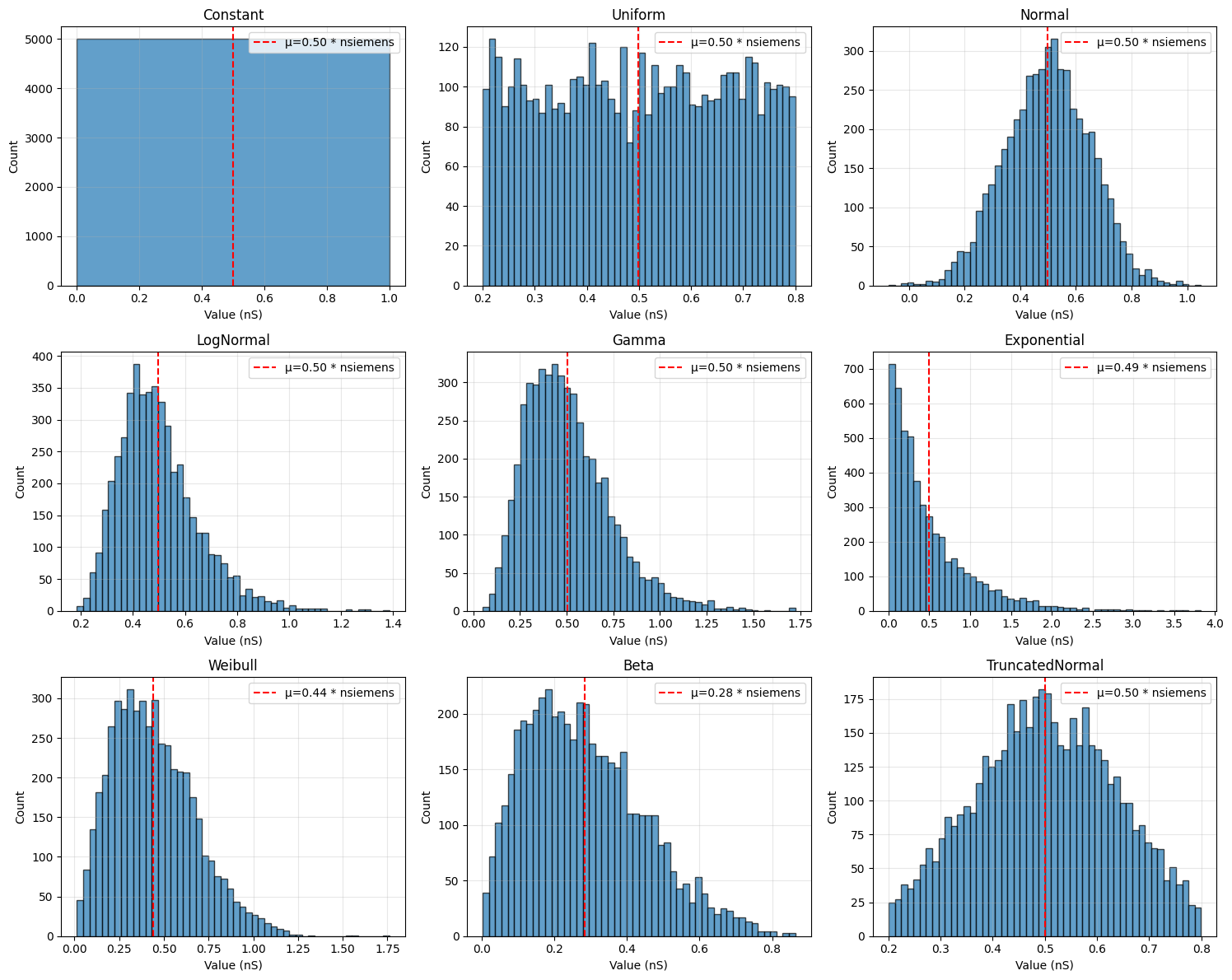
../_images/45c6d346f183b71f5990e05b97ca78e20081d0a3c748062fa8ec8b24755cb79e.png

Statistics Comparison:
--------------------------------------------------------------------------------
Distribution         Mean            Std             Min             Max
--------------------------------------------------------------------------------
Constant             0.5 * nsiemens  0. * nsiemens   0.5 * nsiemens  0.5 * nsiemens
Uniform              0.49923182 * nsiemens 0.17418686 * nsiemens 0.20008174 * nsiemens 0.7998049 * nsiemens
Normal               0.49755648 * nsiemens 0.15192363 * nsiemens -0.07359193 * nsiemens 1.0501068 * nsiemens
LogNormal            0.49728495 * nsiemens 0.15124309 * nsiemens 0.18522009 * nsiemens 1.3853562 * nsiemens
Gamma                0.5038246 * nsiemens 0.22819698 * nsiemens 0.05075649 * nsiemens 1.723785 * nsiemens
Exponential          0.4939349 * nsiemens 0.49528977 * nsiemens 0.00043239 * nsiemens 3.8305352 * nsiemens
Weibull              0.43997285 * nsiemens 0.23112014 * nsiemens 0.01325554 * nsiemens 1.7611426 * nsiemens
Beta                 0.28455865 * nsiemens 0.16196229 * nsiemens 0.00314028 * nsiemens 0.86373866 * nsiemens
TruncatedNormal      0.5008155 * nsiemens 0.13212495 * nsiemens 0.20029485 * nsiemens 0.7995234 * nsiemens

Tutorial 1: Basic Weight Initialization Distributions

Contents

Tutorial 1: Basic Weight Initialization Distributions#

Topics Covered#

Installation and Setup#

1. Introduction to Weight Initialization#

Key Considerations#

2. Basic Distributions: Constant, Uniform, and Normal#

2.1 Constant Initialization#

2.2 Uniform Distribution#

2.3 Normal (Gaussian) Distribution#

Comparing Basic Distributions#

3. Statistical Distributions#

3.1 LogNormal Distribution#

3.2 Gamma Distribution#

3.3 Exponential Distribution#

3.4 Weibull Distribution#

3.5 Beta Distribution#

4. TruncatedNormal Distribution#

Effect of Truncation Bounds#

5. Practical Examples with BrainUnit Quantities#

Example 1: Excitatory and Inhibitory Synaptic Conductances#

Example 2: Spike Rate Parameters#

Example 3: Delay Times with Exponential Distribution#

6. When to Use Each Distribution Type#

Decision Guide#

Comparison Example: All Distributions#