Tutorial 1: Surrogate Gradients for Spiking Neural Networks - Basics

Tutorial 1: Surrogate Gradients for Spiking Neural Networks - Basics#

This tutorial introduces surrogate gradients, a fundamental technique for training spiking neural networks (SNNs). We’ll cover:

What are Surrogate Gradients? - The problem and solution
How Surrogate Gradients Work - The straight-through estimator
Common Surrogate Functions - Overview of popular methods
Visualization & Comparison - Understanding different surrogates
Practical Usage - Using surrogates in SNNs

Setup#

import jax
import jax.numpy as jnp
import matplotlib.pyplot as plt
import numpy as np
import braintools.surrogate as surrogate

# Set up plotting
plt.rcParams['figure.figsize'] = (12, 6)
plt.rcParams['font.size'] = 11

print("Setup complete!")

Setup complete!

1. What are Surrogate Gradients?#

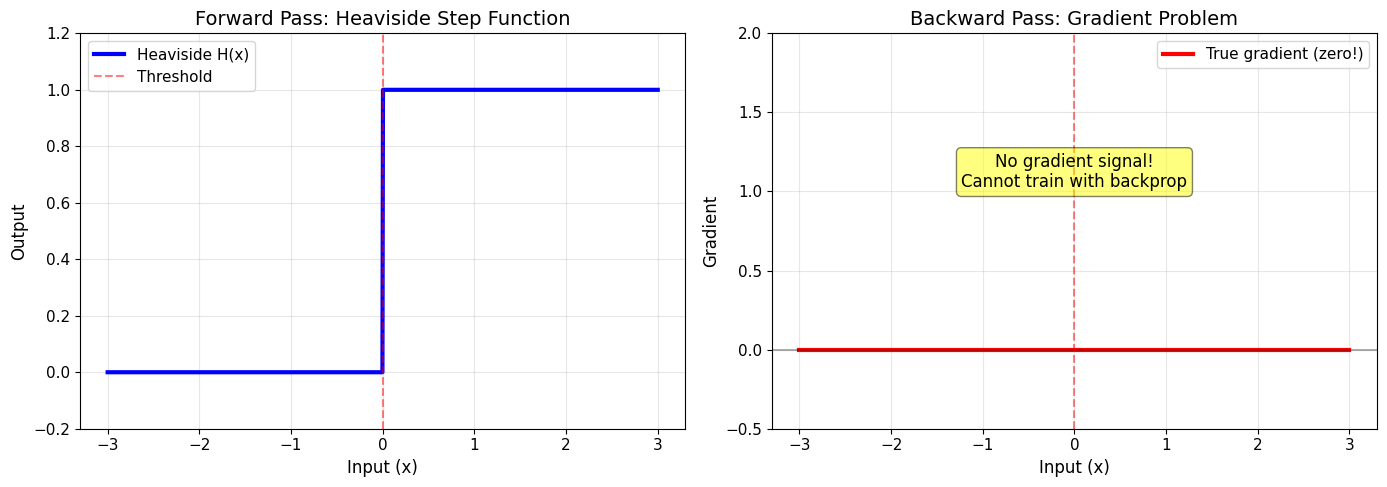
The Problem: Non-Differentiable Spikes#

Spiking neurons produce discrete binary outputs (0 or 1) through a Heaviside step function:

\[\begin{split} s = H(V - V_{\text{th}}) = \begin{cases} 1 & \text{if } V \geq V_{\text{th}} \\ 0 & \text{otherwise} \end{cases} \end{split}\]

The problem: The derivative is zero almost everywhere!

\[\begin{split} \frac{\partial H(x)}{\partial x} = \begin{cases} 0 & \text{if } x \neq 0 \\ \text{undefined} & \text{if } x = 0 \end{cases} \end{split}\]

This means we cannot use gradient descent to train SNNs!

The Solution: Surrogate Gradients#

Surrogate gradients replace the true (zero) gradient with a smooth approximation during backpropagation:

Forward pass: Use the real Heaviside step function $H(x)$
Backward pass: Use a smooth surrogate function $\sigma(x)$ for gradients

This is called the straight-through estimator.

# Demonstrate the problem
print("=== THE GRADIENT PROBLEM ===")

x = jnp.linspace(-3, 3, 1000)

# True Heaviside function
heaviside = jnp.where(x >= 0, 1.0, 0.0)

# Visualize the problem
fig, (ax1, ax2) = plt.subplots(1, 2, figsize=(14, 5))

# Plot Heaviside function
ax1.plot(x, heaviside, 'b-', linewidth=3, label='Heaviside H(x)')
ax1.axvline(0, color='red', linestyle='--', alpha=0.5, label='Threshold')
ax1.set_xlabel('Input (x)', fontsize=12)
ax1.set_ylabel('Output', fontsize=12)
ax1.set_title('Forward Pass: Heaviside Step Function', fontsize=14)
ax1.legend(fontsize=11)
ax1.grid(True, alpha=0.3)
ax1.set_ylim(-0.2, 1.2)

# Plot gradient (which is zero everywhere)
true_gradient = jnp.zeros_like(x)
ax2.plot(x, true_gradient, 'r-', linewidth=3, label='True gradient (zero!)')
ax2.axhline(0, color='black', linestyle='-', alpha=0.3)
ax2.axvline(0, color='red', linestyle='--', alpha=0.5)
ax2.set_xlabel('Input (x)', fontsize=12)
ax2.set_ylabel('Gradient', fontsize=12)
ax2.set_title('Backward Pass: Gradient Problem', fontsize=14)
ax2.legend(fontsize=11)
ax2.grid(True, alpha=0.3)
ax2.set_ylim(-0.5, 2)

# Add text annotations
ax2.text(0, 1, 'No gradient signal!\nCannot train with backprop', 
         ha='center', va='bottom', fontsize=12, 
         bbox=dict(boxstyle='round', facecolor='yellow', alpha=0.5))

plt.tight_layout()
plt.show()

print("\n❌ Problem: The Heaviside function has zero gradient everywhere")
print("❌ This prevents gradient-based learning in SNNs")
print("\n✅ Solution: Use surrogate gradients during backpropagation!")

=== THE GRADIENT PROBLEM ===

../_images/1716aa1c02d24b0807ad6cebe8012149de735f876faa39de1fdc2ef9dc2444d1.png

❌ Problem: The Heaviside function has zero gradient everywhere
❌ This prevents gradient-based learning in SNNs

✅ Solution: Use surrogate gradients during backpropagation!

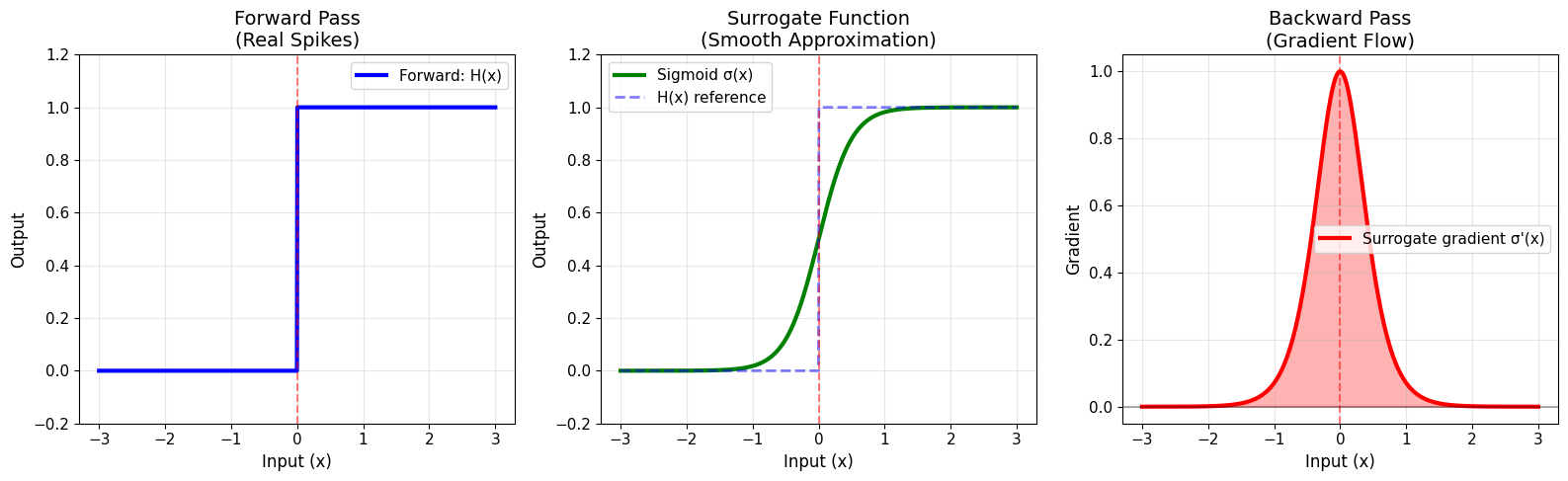
2. How Surrogate Gradients Work#

The straight-through estimator works as follows:

Forward pass: Compute spikes using the real Heaviside function $$s = H(V - V_{\text{th}})$$
Backward pass: Compute gradients using a smooth surrogate $\sigma'(x)$ $$\frac{\partial s}{\partial V} \approx \sigma'(V - V_{\text{th}})$$

This allows gradient flow through the network while maintaining discrete spike outputs!

# Demonstrate surrogate gradient concept
print("=== SURROGATE GRADIENT SOLUTION ===")

# Example: Sigmoid surrogate
sg = surrogate.Sigmoid(alpha=4.0)

x = jnp.linspace(-3, 3, 1000)

# Forward pass (always Heaviside)
forward_output = sg(x)

# Surrogate function (for visualization)
surrogate_function = sg.surrogate_fun(x)

# Surrogate gradient (used in backprop)
surrogate_grad = sg.surrogate_grad(x)

# Visualize the solution
fig, axes = plt.subplots(1, 3, figsize=(16, 5))

# Forward pass
axes[0].plot(x, forward_output, 'b-', linewidth=3, label='Forward: H(x)')
axes[0].axvline(0, color='red', linestyle='--', alpha=0.5)
axes[0].set_xlabel('Input (x)', fontsize=12)
axes[0].set_ylabel('Output', fontsize=12)
axes[0].set_title('Forward Pass\n(Real Spikes)', fontsize=14)
axes[0].legend(fontsize=11)
axes[0].grid(True, alpha=0.3)
axes[0].set_ylim(-0.2, 1.2)

# Surrogate function
axes[1].plot(x, surrogate_function, 'g-', linewidth=3, label='Sigmoid σ(x)')
axes[1].plot(x, forward_output, 'b--', linewidth=2, alpha=0.5, label='H(x) reference')
axes[1].axvline(0, color='red', linestyle='--', alpha=0.5)
axes[1].set_xlabel('Input (x)', fontsize=12)
axes[1].set_ylabel('Output', fontsize=12)
axes[1].set_title('Surrogate Function\n(Smooth Approximation)', fontsize=14)
axes[1].legend(fontsize=11)
axes[1].grid(True, alpha=0.3)
axes[1].set_ylim(-0.2, 1.2)

# Backward pass
axes[2].plot(x, surrogate_grad, 'r-', linewidth=3, label="Surrogate gradient σ'(x)")
axes[2].axvline(0, color='red', linestyle='--', alpha=0.5)
axes[2].axhline(0, color='black', linestyle='-', alpha=0.3)
axes[2].fill_between(x, 0, surrogate_grad, alpha=0.3, color='red')
axes[2].set_xlabel('Input (x)', fontsize=12)
axes[2].set_ylabel('Gradient', fontsize=12)
axes[2].set_title('Backward Pass\n(Gradient Flow)', fontsize=14)
axes[2].legend(fontsize=11)
axes[2].grid(True, alpha=0.3)

plt.tight_layout()
plt.show()

print("\n✅ Forward: Binary spikes (0 or 1)")
print("✅ Backward: Smooth gradients for learning")
print("✅ This enables gradient descent training of SNNs!")

=== SURROGATE GRADIENT SOLUTION ===

../_images/0eeca8d138f1f2508baff9c9b0d9fe91e6c2bbb4d80e6e4c1c7e76eedbbd6751.png

✅ Forward: Binary spikes (0 or 1)
✅ Backward: Smooth gradients for learning
✅ This enables gradient descent training of SNNs!

# Verify gradient computation works
print("=== GRADIENT COMPUTATION DEMONSTRATION ===")

# Create a simple function using surrogate gradient
sg = surrogate.Sigmoid(alpha=4.0)

def spike_function(x):
    return jnp.sum(sg(x))

# Test gradient computation
test_x = jnp.array([0.0])
gradient = jax.grad(spike_function)(test_x)

print(f"Input: {test_x[0]}")
print(f"Forward output (spike): {sg(test_x)[0]}")
print(f"Backward gradient: {gradient[0]:.4f}")
print(f"\n✅ Gradient is non-zero! We can now train with backpropagation.")

# Show how gradient changes with input
x_vals = jnp.linspace(-2, 2, 20)
grads = jax.vmap(lambda x: jax.grad(spike_function)(jnp.array([x]))[0])(x_vals)

plt.figure(figsize=(10, 5))
plt.plot(x_vals, grads, 'o-', linewidth=2, markersize=8, color='purple')
plt.axvline(0, color='red', linestyle='--', alpha=0.5, label='Threshold')
plt.axhline(0, color='black', linestyle='-', alpha=0.3)
plt.xlabel('Input Value', fontsize=12)
plt.ylabel('Gradient', fontsize=12)
plt.title('Gradient Flow Through Surrogate Function', fontsize=14)
plt.legend(fontsize=11)
plt.grid(True, alpha=0.3)
plt.tight_layout()
plt.show()

print("\nNotice: Gradient is strongest near threshold (x=0)!")

=== GRADIENT COMPUTATION DEMONSTRATION ===
Input: 0.0
Forward output (spike): 1.0
Backward gradient: 1.0000

✅ Gradient is non-zero! We can now train with backpropagation.

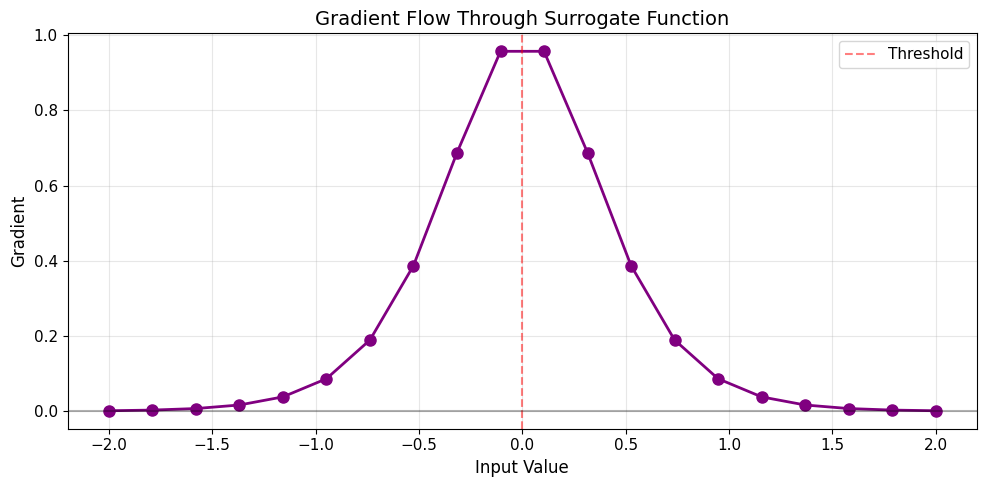
../_images/ab2c95434afc4abc30c54ec832e21c09548d8dd810425b4400aec4ac5c94b697.png

Notice: Gradient is strongest near threshold (x=0)!

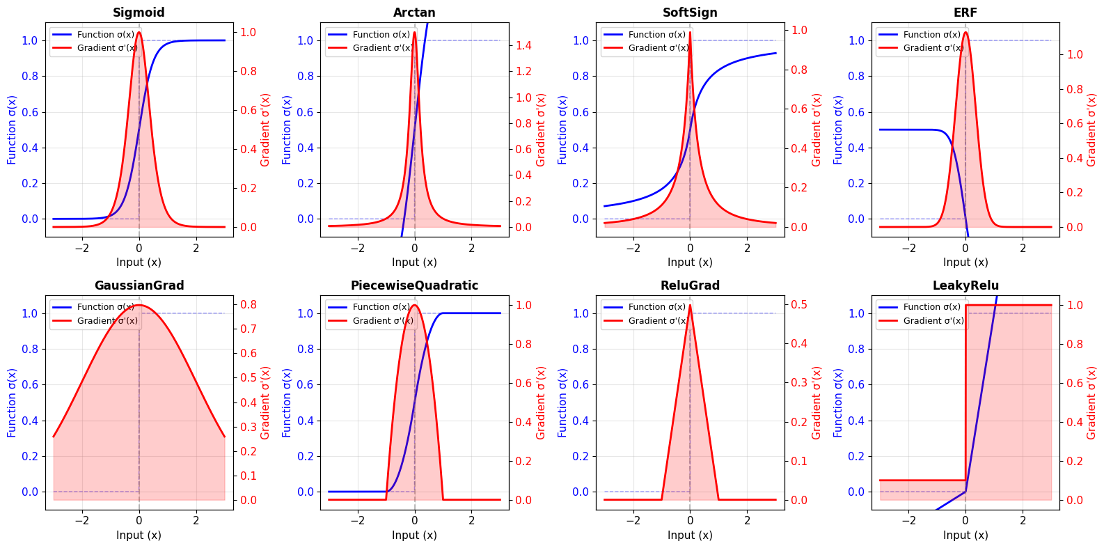
3. Common Surrogate Gradient Functions#

braintools.surrogate provides many surrogate gradient functions. Here are the most popular ones:

Sigmoid-Based Surrogates#

Sigmoid: $\sigma(x) = \frac{1}{1 + e^{-\alpha x}}$, gradient: $\sigma'(x) = \alpha \sigma(x)(1-\sigma(x))$
SoftSign: $\sigma(x) = \frac{x}{1 + |x|}$
Arctan: $\sigma(x) = \frac{1}{\pi}\arctan(\alpha x) + \frac{1}{2}$
ERF: $\sigma(x) = \frac{1}{2}(1 + \text{erf}(\alpha x))$

Piecewise Surrogates#

PiecewiseQuadratic: Quadratic function with finite support
PiecewiseExp: Exponential pieces
PiecewiseLeakyRelu: Leaky ReLU variant

ReLU-Based Surrogates#

ReluGrad: ReLU-inspired with finite support
LeakyRelu: Asymmetric gradients

Distribution-Inspired Surrogates#

GaussianGrad: Gaussian-shaped gradient
MultiGaussianGrad: Multiple Gaussian components
SlayerGrad: From the SLAYER algorithm

Let’s visualize and compare them!

# Compare common surrogate functions
print("=== COMMON SURROGATE GRADIENTS ===")

# Define surrogates to compare
surrogates = {
    'Sigmoid': surrogate.Sigmoid(alpha=4.0),
    'Arctan': surrogate.Arctan(alpha=3.0),
    'SoftSign': surrogate.SoftSign(alpha=2.0),
    'ERF': surrogate.ERF(alpha=2.0),
    'GaussianGrad': surrogate.GaussianGrad(sigma=0.5, alpha=1.0),
    'PiecewiseQuadratic': surrogate.PiecewiseQuadratic(alpha=1.0),
    'ReluGrad': surrogate.ReluGrad(alpha=0.5, width=1.0),
    'LeakyRelu': surrogate.LeakyRelu(alpha=0.1, beta=1.0),
}

x = jnp.linspace(-3, 3, 1000)

# Create subplot grid
n_surrogates = len(surrogates)
n_cols = 4
n_rows = (n_surrogates + n_cols - 1) // n_cols

fig, axes = plt.subplots(n_rows, n_cols, figsize=(16, 4 * n_rows))
axes = axes.flatten()

for idx, (name, sg) in enumerate(surrogates.items()):
    # Plot surrogate function
    ax = axes[idx]
    ax2 = ax.twinx()

    # Function in blue
    try:
        surrogate_fun = sg.surrogate_fun(x)
        line1 = ax.plot(x, surrogate_fun, 'b-', linewidth=2, label='Function σ(x)')
    except NotImplementedError:
        pass
    ax.plot(x, jnp.where(x >= 0, 1.0, 0.0), 'b--', linewidth=1, alpha=0.4, label='H(x)')

    # Gradient in red
    surrogate_grad = sg.surrogate_grad(x)
    line2 = ax2.plot(x, surrogate_grad, 'r-', linewidth=2, label="Gradient σ'(x)")
    ax2.fill_between(x, 0, surrogate_grad, alpha=0.2, color='red')
    
    ax.axvline(0, color='gray', linestyle='--', alpha=0.5)
    ax.set_xlabel('Input (x)')
    ax.set_ylabel('Function σ(x)', color='b')
    ax2.set_ylabel("Gradient σ'(x)", color='r')
    ax.set_title(name, fontsize=12, fontweight='bold')
    ax.tick_params(axis='y', labelcolor='b')
    ax2.tick_params(axis='y', labelcolor='r')
    ax.grid(True, alpha=0.3)
    ax.set_ylim(-0.1, 1.1)
    
    # Combined legend
    lines = line1 + line2
    labels = [l.get_label() for l in lines]
    ax.legend(lines, labels, loc='upper left', fontsize=9)

# Hide extra subplots
for idx in range(len(surrogates), len(axes)):
    axes[idx].axis('off')

plt.tight_layout()
plt.show()

print("\nEach surrogate has different characteristics:")
print("• Sigmoid: Smooth, unbounded support")
print("• Arctan: Smooth, unbounded, moderate steepness")
print("• GaussianGrad: Symmetric, bell-shaped gradient")
print("• PiecewiseQuadratic: Finite support (zero gradient outside range)")
print("• ReluGrad: ReLU-like, finite support")

=== COMMON SURROGATE GRADIENTS ===

../_images/2e55024cba39e22ddfe879037b815f5b848add3881555140c3a5b68ed1adfb63.png

Each surrogate has different characteristics:
• Sigmoid: Smooth, unbounded support
• Arctan: Smooth, unbounded, moderate steepness
• GaussianGrad: Symmetric, bell-shaped gradient
• PiecewiseQuadratic: Finite support (zero gradient outside range)
• ReluGrad: ReLU-like, finite support

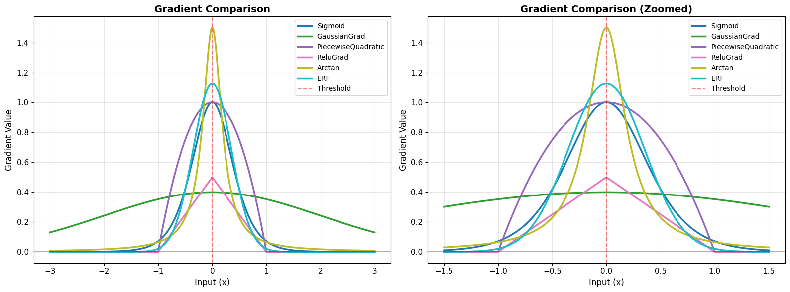
4. Comparing Gradient Shapes#

Different surrogates produce different gradient shapes. Let’s focus on the gradients:

# Compare gradient shapes directly
print("=== GRADIENT SHAPE COMPARISON ===")

# Select representative surrogates
compare_surrogates = [
    ('Sigmoid', surrogate.Sigmoid(alpha=4.0)),
    ('GaussianGrad', surrogate.GaussianGrad(sigma=0.5)),
    ('PiecewiseQuadratic', surrogate.PiecewiseQuadratic(alpha=1.0)),
    ('ReluGrad', surrogate.ReluGrad(alpha=0.5, width=1.0)),
    ('Arctan', surrogate.Arctan(alpha=3.0)),
    ('ERF', surrogate.ERF(alpha=2.0)),
]

x = jnp.linspace(-3, 3, 1000)

fig, (ax1, ax2) = plt.subplots(1, 2, figsize=(16, 6))

# Plot all gradients together
colors = plt.cm.tab10(np.linspace(0, 1, len(compare_surrogates)))

for idx, (name, sg) in enumerate(compare_surrogates):
    grad = sg.surrogate_grad(x)
    ax1.plot(x, grad, linewidth=2.5, label=name, color=colors[idx])

ax1.axvline(0, color='red', linestyle='--', alpha=0.5, label='Threshold')
ax1.axhline(0, color='black', linestyle='-', alpha=0.3)
ax1.set_xlabel('Input (x)', fontsize=12)
ax1.set_ylabel('Gradient Value', fontsize=12)
ax1.set_title('Gradient Comparison', fontsize=14, fontweight='bold')
ax1.legend(fontsize=10, loc='upper right')
ax1.grid(True, alpha=0.3)

# Plot gradient width comparison (zoomed)
x_zoom = jnp.linspace(-1.5, 1.5, 1000)

for idx, (name, sg) in enumerate(compare_surrogates):
    grad = sg.surrogate_grad(x_zoom)
    ax2.plot(x_zoom, grad, linewidth=2.5, label=name, color=colors[idx])

ax2.axvline(0, color='red', linestyle='--', alpha=0.5, label='Threshold')
ax2.axhline(0, color='black', linestyle='-', alpha=0.3)
ax2.set_xlabel('Input (x)', fontsize=12)
ax2.set_ylabel('Gradient Value', fontsize=12)
ax2.set_title('Gradient Comparison (Zoomed)', fontsize=14, fontweight='bold')
ax2.legend(fontsize=10, loc='upper right')
ax2.grid(True, alpha=0.3)

plt.tight_layout()
plt.show()

print("\nKey observations:")
print("• GaussianGrad: Narrow, peaked gradient")
print("• Sigmoid/Arctan/ERF: Medium width, smooth decay")
print("• PiecewiseQuadratic/ReluGrad: Finite support (hard cutoff)")
print("\nChoice impacts:")
print("• Narrow gradients: More selective, faster convergence")
print("• Wide gradients: More gradient flow, more stable")

=== GRADIENT SHAPE COMPARISON ===

../_images/e2652c8d5731fe2ccade4f0d5872fe02495beb41ba815258b822b07d66d10587.png

Key observations:
• GaussianGrad: Narrow, peaked gradient
• Sigmoid/Arctan/ERF: Medium width, smooth decay
• PiecewiseQuadratic/ReluGrad: Finite support (hard cutoff)

Choice impacts:
• Narrow gradients: More selective, faster convergence
• Wide gradients: More gradient flow, more stable

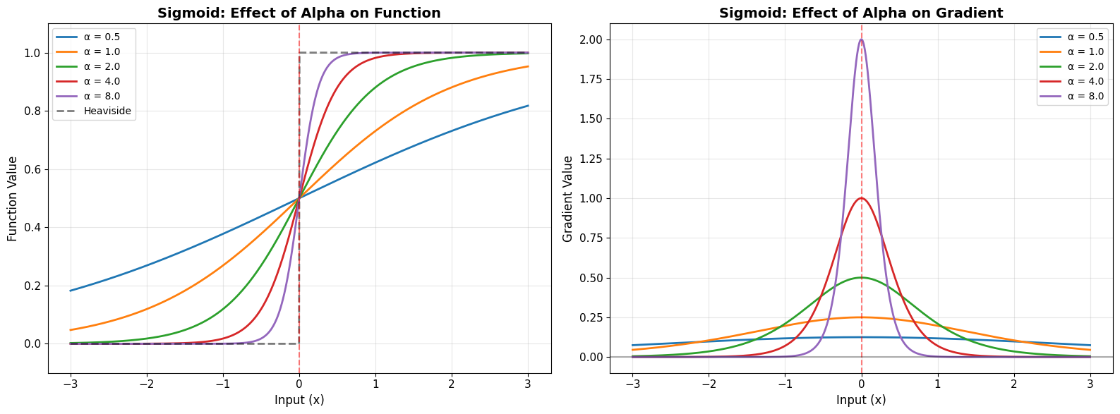
5. Effect of Hyperparameters#

Most surrogate functions have a steepness parameter (usually called alpha) that controls the shape of the gradient.

# Demonstrate effect of alpha parameter
print("=== HYPERPARAMETER EFFECTS: Alpha ===")

alphas = [0.5, 1.0, 2.0, 4.0, 8.0]
x = jnp.linspace(-3, 3, 1000)

fig, axes = plt.subplots(1, 2, figsize=(16, 6))

# Sigmoid example
for alpha in alphas:
    sg = surrogate.Sigmoid(alpha=alpha)
    surrogate_fun = sg.surrogate_fun(x)
    axes[0].plot(x, surrogate_fun, linewidth=2, label=f'α = {alpha}')

axes[0].plot(x, jnp.where(x >= 0, 1.0, 0.0), 'k--', linewidth=2, alpha=0.5, label='Heaviside')
axes[0].axvline(0, color='red', linestyle='--', alpha=0.5)
axes[0].set_xlabel('Input (x)', fontsize=12)
axes[0].set_ylabel('Function Value', fontsize=12)
axes[0].set_title('Sigmoid: Effect of Alpha on Function', fontsize=14, fontweight='bold')
axes[0].legend(fontsize=10)
axes[0].grid(True, alpha=0.3)
axes[0].set_ylim(-0.1, 1.1)

# Gradients
for alpha in alphas:
    sg = surrogate.Sigmoid(alpha=alpha)
    grad = sg.surrogate_grad(x)
    axes[1].plot(x, grad, linewidth=2, label=f'α = {alpha}')

axes[1].axvline(0, color='red', linestyle='--', alpha=0.5)
axes[1].axhline(0, color='black', linestyle='-', alpha=0.3)
axes[1].set_xlabel('Input (x)', fontsize=12)
axes[1].set_ylabel('Gradient Value', fontsize=12)
axes[1].set_title('Sigmoid: Effect of Alpha on Gradient', fontsize=14, fontweight='bold')
axes[1].legend(fontsize=10)
axes[1].grid(True, alpha=0.3)

plt.tight_layout()
plt.show()

print("\nEffect of increasing α:")
print("• Surrogate function becomes steeper (closer to Heaviside)")
print("• Gradient becomes narrower and taller")
print("• Peak gradient value increases")
print("\nTrade-off:")
print("• High α: More accurate approximation, but narrower gradient flow")
print("• Low α: Wider gradient flow, but less accurate approximation")

=== HYPERPARAMETER EFFECTS: Alpha ===

../_images/54d371863f413676d83c0823a1f8de3739bf0573dfdb74ec6c6231b06b3efc4c.png

Effect of increasing α:
• Surrogate function becomes steeper (closer to Heaviside)
• Gradient becomes narrower and taller
• Peak gradient value increases

Trade-off:
• High α: More accurate approximation, but narrower gradient flow
• Low α: Wider gradient flow, but less accurate approximation

6. Practical Usage in SNNs#

Let’s see how to use surrogate gradients in a simple spiking neuron model.

# Simple LIF neuron with surrogate gradient
print("=== PRACTICAL EXAMPLE: LIF Neuron ===")

# LIF neuron parameters
tau = 10.0  # membrane time constant (ms)
v_th = 1.0  # threshold voltage
dt = 0.1    # time step (ms)

# Choose surrogate gradient
spike_grad = surrogate.Sigmoid(alpha=4.0)

def lif_step(v, i_input):
    """Single step of LIF neuron dynamics."""
    # Update membrane potential
    dv = (-v + i_input) / tau * dt
    v = v + dv
    
    # Generate spike with surrogate gradient
    spike = spike_grad(v - v_th)
    
    # Reset after spike
    v = v * (1.0 - spike)
    
    return v, spike

# Simulate neuron
n_steps = 500
i_input = jnp.ones(n_steps) * 1.5  # Constant input current

v_trace = []
spike_trace = []
v = jnp.array(0.0)

for i in range(n_steps):
    v, spike = lif_step(v, i_input[i])
    v_trace.append(float(v))
    spike_trace.append(float(spike))

v_trace = jnp.array(v_trace)
spike_trace = jnp.array(spike_trace)
time = jnp.arange(n_steps) * dt

# Plot results
fig, (ax1, ax2) = plt.subplots(2, 1, figsize=(14, 8))

# Membrane potential
ax1.plot(time, v_trace, 'b-', linewidth=2, label='Membrane potential')
ax1.axhline(v_th, color='red', linestyle='--', linewidth=2, label='Threshold')
spike_times = time[spike_trace > 0.5]
ax1.scatter(spike_times, jnp.ones_like(spike_times) * v_th, 
           color='red', s=100, zorder=5, label='Spikes', marker='^')
ax1.set_ylabel('Membrane Potential (V)', fontsize=12)
ax1.set_title('LIF Neuron with Surrogate Gradient', fontsize=14, fontweight='bold')
ax1.legend(fontsize=11)
ax1.grid(True, alpha=0.3)

# Spikes
ax2.eventplot(spike_times, lineoffsets=0.5, linelengths=0.8, linewidths=2, color='red')
ax2.set_xlabel('Time (ms)', fontsize=12)
ax2.set_ylabel('Spike', fontsize=12)
ax2.set_ylim(0, 1)
ax2.set_yticks([0, 1])
ax2.set_yticklabels(['No', 'Yes'])
ax2.set_title('Spike Train Output', fontsize=14, fontweight='bold')
ax2.grid(True, alpha=0.3)

plt.tight_layout()
plt.show()

print(f"\nSimulation results:")
print(f"• Total spikes: {jnp.sum(spike_trace > 0.5):.0f}")
print(f"• Firing rate: {jnp.sum(spike_trace > 0.5) / (n_steps * dt) * 1000:.1f} Hz")
print(f"\n✅ Spikes are discrete (0 or 1) in forward pass")
print(f"✅ But gradients flow through via surrogate function!")

=== PRACTICAL EXAMPLE: LIF Neuron ===

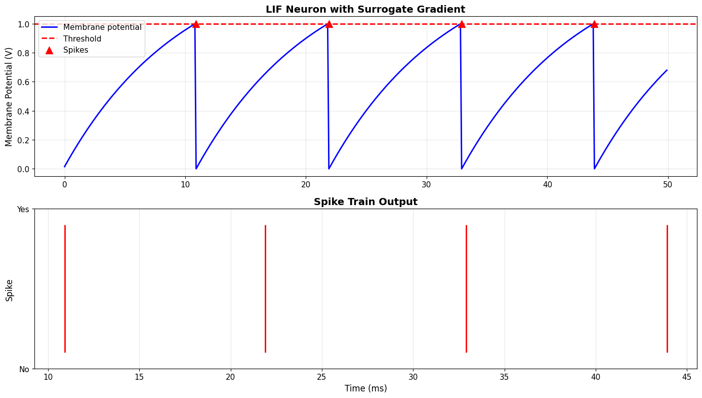
../_images/77348a16483b98b6837de4e1a37304fdbe92edd3d832a53a7216d1ba0748033b.png

Simulation results:
• Total spikes: 4
• Firing rate: 80.0 Hz

✅ Spikes are discrete (0 or 1) in forward pass
✅ But gradients flow through via surrogate function!

# Demonstrate gradient flow through neuron
print("=== GRADIENT FLOW DEMONSTRATION ===")

def neuron_output(i_input_value):
    """Compute total spikes for given input."""
    v = jnp.array(0.0)
    total_spikes = 0.0
    
    for _ in range(100):
        dv = (-v + i_input_value) / tau * dt
        v = v + dv
        spike = spike_grad(v - v_th)
        total_spikes = total_spikes + spike
        v = v * (1.0 - spike)
    
    return total_spikes

# Compute gradient of output w.r.t. input current
test_currents = jnp.linspace(0.5, 2.5, 50)
outputs = jax.vmap(neuron_output)(test_currents)
gradients = jax.vmap(jax.grad(neuron_output))(test_currents)

fig, (ax1, ax2) = plt.subplots(1, 2, figsize=(16, 5))

# Input-output relationship
ax1.plot(test_currents, outputs, 'bo-', linewidth=2, markersize=6)
ax1.set_xlabel('Input Current', fontsize=12)
ax1.set_ylabel('Total Spikes (100 steps)', fontsize=12)
ax1.set_title('Neuron Input-Output Function', fontsize=14, fontweight='bold')
ax1.grid(True, alpha=0.3)

# Gradient of output w.r.t. input
ax2.plot(test_currents, gradients, 'ro-', linewidth=2, markersize=6)
ax2.axhline(0, color='black', linestyle='-', alpha=0.3)
ax2.set_xlabel('Input Current', fontsize=12)
ax2.set_ylabel('Gradient (∂spikes/∂current)', fontsize=12)
ax2.set_title('Gradient Flow', fontsize=14, fontweight='bold')
ax2.grid(True, alpha=0.3)

plt.tight_layout()
plt.show()

print("\n✅ Gradient successfully flows through spiking neuron!")
print("✅ This enables learning in SNNs via backpropagation")
print(f"\nGradient statistics:")
print(f"• Mean gradient: {jnp.mean(gradients):.4f}")
print(f"• Max gradient: {jnp.max(gradients):.4f}")
print(f"• Min gradient: {jnp.min(gradients):.4f}")

=== GRADIENT FLOW DEMONSTRATION ===

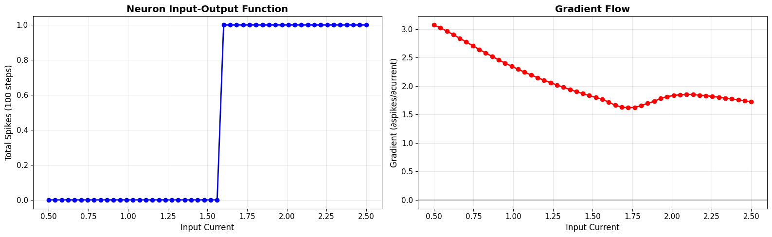
../_images/e95d730649220cb54711833d2d62bf207a4f318970bf1bc71fa8babc4c89602f.png

✅ Gradient successfully flows through spiking neuron!
✅ This enables learning in SNNs via backpropagation

Gradient statistics:
• Mean gradient: 2.0763
• Max gradient: 3.0740
• Min gradient: 1.6188

7. Choosing the Right Surrogate#

Different surrogates work better for different tasks. Here’s a quick guide:

Recommended Surrogates#

Surrogate	When to Use	Pros	Cons
Sigmoid	General purpose, default choice	Smooth, well-studied	Unbounded support
Arctan	Similar to Sigmoid	Smoother than sigmoid	Slower computation
GaussianGrad	Need precise gradient control	Symmetric, peaked	Requires sigma tuning
PiecewiseQuadratic	Memory efficiency important	Finite support, fast	Less smooth
ReluGrad	Deep SNNs	Finite support, stable	May need tuning
SuperSpike (GaussianGrad)	Research baseline	Well-studied	Standard choice

General Guidelines#

Start with Sigmoid (α=4.0): Good default for most tasks
Use GaussianGrad for precise control: Popular in research
Try PiecewiseQuadratic for efficiency: Finite support saves memory
Experiment with α: Tune steepness for your specific task

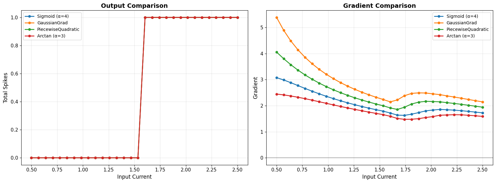
Performance Comparison#

# Compare different surrogates on the same task
print("=== SURROGATE COMPARISON ON LIF NEURON ===")

surrogates_to_test = {
    'Sigmoid (α=4)': surrogate.Sigmoid(alpha=4.0),
    'GaussianGrad': surrogate.GaussianGrad(sigma=0.5, alpha=1.0),
    'PiecewiseQuadratic': surrogate.PiecewiseQuadratic(alpha=1.0),
    'Arctan (α=3)': surrogate.Arctan(alpha=3.0),
}

test_currents = jnp.linspace(0.5, 2.5, 30)

fig, axes = plt.subplots(1, 2, figsize=(16, 6))

for name, sg in surrogates_to_test.items():
    def neuron_with_surrogate(i_input_value):
        v = jnp.array(0.0)
        total_spikes = 0.0
        for _ in range(100):
            v = v + (-v + i_input_value) / tau * dt
            spike = sg(v - v_th)
            total_spikes = total_spikes + spike
            v = v * (1.0 - spike)
        return total_spikes
    
    outputs = jax.vmap(neuron_with_surrogate)(test_currents)
    gradients = jax.vmap(jax.grad(neuron_with_surrogate))(test_currents)
    
    axes[0].plot(test_currents, outputs, 'o-', linewidth=2, markersize=5, label=name)
    axes[1].plot(test_currents, gradients, 'o-', linewidth=2, markersize=5, label=name)

axes[0].set_xlabel('Input Current', fontsize=12)
axes[0].set_ylabel('Total Spikes', fontsize=12)
axes[0].set_title('Output Comparison', fontsize=14, fontweight='bold')
axes[0].legend(fontsize=10)
axes[0].grid(True, alpha=0.3)

axes[1].set_xlabel('Input Current', fontsize=12)
axes[1].set_ylabel('Gradient', fontsize=12)
axes[1].set_title('Gradient Comparison', fontsize=14, fontweight='bold')
axes[1].legend(fontsize=10)
axes[1].grid(True, alpha=0.3)
axes[1].axhline(0, color='black', linestyle='-', alpha=0.3)

plt.tight_layout()
plt.show()

print("\nObservations:")
print("• All surrogates produce same forward behavior (spikes)")
print("• Different gradient magnitudes and shapes")
print("• Choice affects learning dynamics, not output")

=== SURROGATE COMPARISON ON LIF NEURON ===

../_images/3b1e82f3bbc30e65fafe1eda5493cc8e4649558033c9852bad55326f379ee8b3.png

Observations:
• All surrogates produce same forward behavior (spikes)
• Different gradient magnitudes and shapes
• Choice affects learning dynamics, not output