Coupling and Delays

A whole-brain model is more than a collection of independent regions — it is a network. This page explains the three ingredients that wire regions together: the structural connectivity (who connects to whom), the conduction delays (how long a signal takes to travel), and the coupling function (how a neighbour’s activity enters a region’s dynamics). It covers the maths and the intuition; the hands-on recipe is Custom Coupling, and the API is brainmass.Network and the *Coupling classes.

Structural connectivity (SC)

The wiring diagram of a brain network is a structural connectivity matrix \(W \in \mathbb{R}^{N \times N}\) for \(N\) regions. Each entry \(W_{ij}\) is the strength of the anatomical connection from region \(j\) to region \(i\), typically estimated from diffusion-MRI tractography (streamline counts between parcels) or taken from a tract-tracing atlas.

Conventions that matter in practice:

• No self-connections. The diagonal \(W_{ii}\) is usually zeroed — a region’s recurrent dynamics live inside its own neural mass model, not in the SC. brainmass.Network zeroes the diagonal for you (unless you opt in with self_connection=True).

• Weights are non-negative and often normalised (e.g. to \([0,1]\), or row-/ Laplacian-normalised). A global scalar \(k\) (TVB calls it \(G\); brainmass keeps the convention \(G \equiv k\)) sets the overall coupling strength on top of \(W\).

• Symmetry is common for diffusion-MRI SC (tractography is undirected) but not required; directed connectomes are supported.

The bundled datasets.load_dataset('example_connectome') provides a small symmetric \(8 \times 8\) \(W\) (plus a distance matrix) to experiment with.

Conduction delays

Axons conduct at a finite speed, so a signal leaving region \(j\) arrives at region \(i\) only after a conduction delay

\[ \tau_{ij} \;=\; \frac{d_{ij}}{v}, \]

where \(d_{ij}\) is the fibre length between the regions (a distance matrix, often in mm) and \(v\) is the conduction speed (mm/ms, typically a few m/s for myelinated white-matter tracts). Delays are essential: they are what let a network of identical oscillators produce travelling waves, metastable switching, and realistic resting-state dynamics rather than collapsing to global synchrony.

With delays, the coupling that region \(i\) feels at time \(t\) reads the past state of its sources:

\[ \text{input}_i(t) \;\propto\; \sum_j W_{ij}\, x_j\!\left(t - \tau_{ij}\right). \]

Numerically this needs a delay buffer — a ring buffer of recent history sized from \(\max_{ij}\tau_{ij} / \Delta t\) steps. brainmass builds this for you when you pass distance and speed to Network; if either is omitted the coupling is instantaneous (zero delays). Units are handled automatically: if distance carries length units and speed carries length/time units, the delay is unit-correct; plain numbers are assumed to be milliseconds. The self-delay (the diagonal of \(\tau\)) is always zeroed.

One practical wrinkle: Network sizes its delay buffer from the global dt at construction time, so set brainstate.environ.set(dt=…) before building a delay-coupled network. The Simulator then drives it with that same dt.

How activity enters a region: three coupling functions

Given the (possibly delayed) source activity and the SC, a coupling function turns them into the current that drives each region. brainmass provides three families. The choice is a modelling decision with real dynamical consequences.

Diffusive coupling

Diffusive coupling drives a region by the difference between its neighbours’ activity and its own:

\[ \text{current}_i \;=\; k \sum_j W_{ij}\,\bigl(x_j^{(\tau)} - y_i\bigr), \]

where \(x_j^{(\tau)}\) is the delayed source state of region \(j\) and \(y_i\) is the target region’s own state. This is the discrete graph-Laplacian form: it is relative, vanishes when all regions agree (\(x_j = y_i\)), and tends to pull connected regions toward a common value — it is the natural model of an electrotonic / gap-junction-like interaction and the most common choice for whole-brain models. It is brainmass’s default (coupling='diffusive').

import brainmass
import jax.numpy as jnp

# Diffusive coupling current for a tiny 2-region example, by hand.
W = jnp.array([[0.0, 1.0],
               [1.0, 0.0]])      # symmetric, zero diagonal
x = jnp.array([[1.0, 2.0],       # source-as-seen-by-target matrix (N_out, N_in)
               [1.0, 2.0]])
y = jnp.array([1.0, 2.0])        # each region's own state
k = 0.5

current = brainmass.diffusive_coupling(x, y, W, k)
print('diffusive current per region:', current)   # k * sum_j W_ij (x_j - y_i)

diffusive current per region: [ 0.5 -0.5]

Additive (linear) coupling

Additive coupling simply injects a weighted sum of the neighbours’ activity, with no subtraction of the target’s own state:

\[ \text{current}_i \;=\; k \sum_j W_{ij}\,x_j^{(\tau)} \;+\; b. \]

This is absolute rather than relative: a region keeps receiving drive even when it already matches its neighbours, so additive coupling does not vanish at consensus. It corresponds to TVB’s Linear coupling; the optional bias \(b\) shifts the operating point. Use it when a neighbour’s activity should act as a direct synaptic input (e.g. excitatory drive) rather than a pull toward agreement. Select it with coupling='additive'.

Nonlinear coupling

Real synaptic transmission saturates: a presynaptic rate maps to a bounded postsynaptic effect through a sigmoid. Nonlinear couplings apply a saturating function and split on where the nonlinearity sits.

Post-nonlinearity (the function is applied to the summed network input):

\[ c_i \;=\; k\,\sigma\!\Bigl(\text{slope}\cdot\bigl(a\textstyle\sum_j W_{ij}x_j + b - \text{midpoint}\bigr)\Bigr) \quad\text{(sigmoidal)}, \qquad c_i \;=\; k\,\tanh\!\Bigl(\text{scale}\textstyle\sum_j W_{ij}x_j\Bigr) \quad\text{(hyperbolic tangent)}. \]

Pre-nonlinearity (each source is passed through the nonlinearity before weighting — the Jansen–Rit convention):

\[ c_i \;=\; k\sum_j W_{ij}\,\sigma_{\mathrm{JR}}(x_j), \qquad \sigma_{\mathrm{JR}}(x) = c_{\min} + \frac{c_{\max}-c_{\min}}{1 + e^{\,r(\text{midpoint}-x)}}. \]

The post-/pre- distinction is the key design axis: post-forms saturate the total incoming drive (the output carries \(k\)’s unit); the pre-form saturates each source firing rate into a synaptic effect before summation. brainmass exposes these as coupling='sigmoidal' | 'tanh' | 'sigmoidal_jansen_rit', and the tanh saturation is easy to see directly.

import brainmass
import jax.numpy as jnp

W = jnp.ones((2, 2))
k, scale = 0.5, 2.0

# tanh coupling saturates to +/- k as the network input grows.
for level in (0.1, 1.0, 5.0):
    x = jnp.full((2, 2), level)
    c = brainmass.hyperbolic_tangent_coupling(x, W, k=k, scale=scale)
    print(f'input level {level:>4}: coupling current {c[0]:.4f}  (saturates toward k={k})')

input level  0.1: coupling current 0.1900  (saturates toward k=0.5)
input level  1.0: coupling current 0.4997  (saturates toward k=0.5)
input level  5.0: coupling current 0.5000  (saturates toward k=0.5)

Notice how the current flattens toward \(k = 0.5\) as the input grows — the bounded synaptic response that linear coupling lacks. (Through Network, the nonlinear kernels use their default shape parameters; to tune slope / scale / midpoint build the coupling class directly, e.g. HyperbolicTangentCoupling(...).)

A small illustrative network

Putting it together: an 8-region network of Hopf oscillators, wired by the bundled example connectome, with distance-dependent conduction delays and diffusive coupling. This is the full SC → coupling + delays → activity pipeline in a few lines. The Simulator drives the Network exactly like a single node.

import brainmass
import brainstate
import brainunit as u

brainstate.random.seed(0)
brainstate.environ.set(dt=0.1 * u.ms)   # set BEFORE building a delayed Network

conn = brainmass.datasets.load_dataset('example_connectome')
node = brainmass.HopfStep(in_size=conn.weights.shape[0], a=0.2, w=0.3)

net = brainmass.Network(
    node,
    conn=conn.weights,            # structural connectivity W (diagonal zeroed)
    distance=conn.distances,      # fibre lengths (mm)
    speed=10.0 * u.mm / u.ms,     # conduction speed -> delays = distance / speed
    coupling='diffusive',
    coupled_var='x',              # coupling current drives the x variable
    k=0.5,                        # global coupling strength (== TVB's G)
)

res = brainmass.Simulator(net, dt=0.1 * u.ms).run(
    400 * u.ms, monitors=lambda m: m.node.x.value, transient=100 * u.ms)
print('network output (time x regions):', res['output'].shape)

network output (time x regions): (3000, 8)

import matplotlib.pyplot as plt

fig, (ax1, ax2) = plt.subplots(1, 2, figsize=(11, 4))

# The structural connectivity that wired the network.
brainmass.viz.plot_connectivity(conn.weights, labels=list(conn.labels), ax=ax1)
ax1.set_title('Structural connectivity $W$')

# The resulting coupled regional activity.
brainmass.viz.plot_timeseries(res['output'], ts=res['ts'], ax=ax2)
ax2.set_title('Delay-coupled regional activity')

fig.tight_layout()
plt.show()

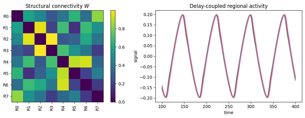
The left panel is the anatomy (\(W\)); the right is the dynamics it produces once the regions are coupled with conduction delays. Change \(k\), the speed, or the coupling function and the collective behaviour — synchrony, metastability, travelling patterns — changes with it. Exploring that map from wiring to dynamics is much of what whole-brain modelling is about.

Key takeaways

• Structural connectivity \(W\) is the wiring diagram; zero its diagonal and scale it by a global strength \(k\) (\(\equiv\) TVB’s \(G\)).

• Conduction delays \(\tau_{ij} = d_{ij}/v\) come from a distance matrix and a finite speed; they are essential for realistic large-scale dynamics and need a delay buffer (built automatically by Network).

• Diffusive coupling is relative (a Laplacian pull toward consensus), additive is absolute (direct injected drive), and nonlinear couplings add synaptic saturation, split into post- and pre-nonlinearity forms.

See also

• Custom Coupling — swapping coupling functions in practice.

• Building a Network — building a connectome network step by step.

• Architecture Overview — where Network sits in the package.

• What Is a Neural Mass Model? — the per-region nodes being coupled.

References

• Sanz-Leon, P., Knock, S. A., Spiegler, A., & Jirsa, V. K. (2015). Mathematical framework for large-scale brain network modeling in The Virtual Brain. NeuroImage, 111, 385–430.

• Deco, G., Jirsa, V., McIntosh, A. R., Sporns, O., & Kötter, R. (2009). Key role of coupling, delay, and noise in resting brain fluctuations. PNAS, 106(25), 10302–10307.

• Honey, C. J., et al. (2009). Predicting human resting-state functional connectivity from structural connectivity. PNAS, 106(6), 2035–2040.