Run Parameter Sweeps

Goal: evaluate a model over a grid of parameter values, collect the results into a tidy table, and visualize them as a heatmap.

The idiom is a single brainstate.transform.vmap over a function that builds the model inside itself — one simulation per grid point, all fused into one compiled program. No Python loop over parameters, no manual batching.

1-D sweep

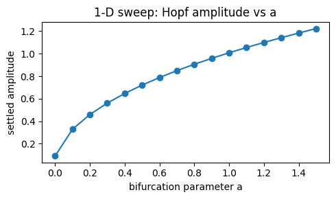
Start with one parameter. We sweep the Hopf bifurcation parameter a and measure the settled limit-cycle amplitude (a scalar summary — see Fitting with Gradients for why scalar summaries beat raw time series for oscillators).

The pattern: write run_one(a) that constructs the model with that a, runs a Simulator, and returns a scalar; then vmap it over the value array.

def amplitude_for(a):
    node = brainmass.HopfStep(in_size=1, a=a, w=0.3,
                              init_x=braintools.init.Constant(0.5))
    res = brainmass.Simulator(node, dt=0.1 * u.ms).run(
        150 * u.ms, monitors=['x'], transient=50 * u.ms)
    x = u.get_magnitude(res['x'])[:, 0]
    return jnp.sqrt(jnp.mean(x ** 2)) * jnp.sqrt(2.0)  # RMS limit-cycle amplitude

a_values = jnp.linspace(0.0, 1.5, 16)
amps = brainstate.transform.vmap(amplitude_for)(a_values)
print("swept", len(a_values), "values in one vmap call")

swept 16 values in one vmap call

Plot the sweep. The amplitude grows like √a past the bifurcation at a = 0, the signature of a supercritical Hopf.

fig, ax = plt.subplots(figsize=(5, 3))
ax.plot(np.asarray(a_values), np.asarray(amps), 'o-')
ax.set_xlabel('bifurcation parameter a')
ax.set_ylabel('settled amplitude')
ax.set_title('1-D sweep: Hopf amplitude vs a')
fig.tight_layout()
plt.show()

2-D sweep → tidy table

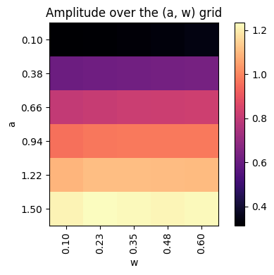
For two parameters, build a mesh, flatten it, vmap over the flattened pairs, then reshape the result back to the grid. Here we sweep a (bifurcation) against w (intrinsic frequency).

brainstate.transform.vmap maps over the leading axis of each argument, so we pass the two flattened coordinate arrays.

a_grid = jnp.linspace(0.1, 1.5, 6)
w_grid = jnp.linspace(0.1, 0.6, 5)
AA, WW = jnp.meshgrid(a_grid, w_grid, indexing='ij')

def amplitude_aw(a, w):
    node = brainmass.HopfStep(in_size=1, a=a, w=w,
                              init_x=braintools.init.Constant(0.5))
    res = brainmass.Simulator(node, dt=0.1 * u.ms).run(
        150 * u.ms, monitors=['x'], transient=50 * u.ms)
    x = u.get_magnitude(res['x'])[:, 0]
    return jnp.sqrt(jnp.mean(x ** 2)) * jnp.sqrt(2.0)

amp_flat = brainstate.transform.vmap(amplitude_aw)(AA.reshape(-1), WW.reshape(-1))
amp_grid = np.asarray(amp_flat).reshape(AA.shape)
print("grid shape:", amp_grid.shape, "(len(a), len(w))")

grid shape: (6, 5) (len(a), len(w))

Collect the results into a tidy, long-format table. We use a plain dict of columns (numpy) so there is no hard pandas dependency; convert to a pandas.DataFrame in one line if you have it installed.

table = {
    'a': np.asarray(AA).reshape(-1),
    'w': np.asarray(WW).reshape(-1),
    'amplitude': np.asarray(amp_flat),
}

# Pretty-print the first few rows (pandas optional: pd.DataFrame(table)).
print(f"{'a':>6} {'w':>6} {'amplitude':>10}")
for i in range(8):
    print(f"{table['a'][i]:6.2f} {table['w'][i]:6.2f} {table['amplitude'][i]:10.3f}")
print(f"... ({len(table['a'])} rows total)")

     a      w  amplitude
  0.10   0.10      0.313
  0.10   0.23      0.318
  0.10   0.35      0.325
  0.10   0.48      0.333
  0.10   0.60      0.343
  0.38   0.10      0.609
  0.38   0.23      0.615
  0.38   0.35      0.621
... (30 rows total)

Heatmap

Visualize the 2-D grid with brainmass.viz.plot_connectivity (it draws any matrix as a labelled heatmap with a colorbar — not just connectomes). The amplitude depends almost entirely on a (the bifurcation parameter), so the heatmap shows horizontal bands.

fig, ax = plt.subplots(figsize=(5, 4))
brainmass.viz.plot_connectivity(
    amp_grid, ax=ax, cmap='magma',
    labels=None,
)
ax.set_xlabel('w index')
ax.set_ylabel('a index')
ax.set_title('Amplitude over the (a, w) grid')
# annotate the real axis values
ax.set_xticks(range(len(w_grid)))
ax.set_xticklabels([f'{float(w):.2f}' for w in w_grid], rotation=90)
ax.set_yticks(range(len(a_grid)))
ax.set_yticklabels([f'{float(a):.2f}' for a in a_grid])
ax.set_xlabel('w')
ax.set_ylabel('a')
fig.tight_layout()
plt.show()

Sweeping a network coupling

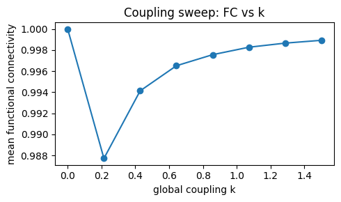
The same pattern sweeps a network parameter. Here we vary the global coupling strength k of a diffusive Network and measure the mean functional-connectivity strength — a standard way to find the coupling regime that best matches data.

conn = brainmass.datasets.load_dataset('example_connectome')
W, D, N = conn.weights, conn.distances, conn.weights.shape[0]

def mean_fc_for(k):
    node = brainmass.HopfStep(in_size=N, a=0.2, w=0.3,
                              init_x=braintools.init.Constant(0.3))
    net = brainmass.Network(node, conn=W, distance=D, speed=10 * u.mm / u.ms,
                            coupling='diffusive', coupled_var='x', k=k)
    res = brainmass.Simulator(net, dt=0.1 * u.ms).run(
        600 * u.ms, monitors=lambda m: m.node.x.value, transient=100 * u.ms)
    sig = u.get_magnitude(res['output'])
    fc = braintools.metric.functional_connectivity(sig)
    iu = np.triu_indices(N, 1)
    return jnp.mean(fc[iu])

k_values = jnp.linspace(0.0, 1.5, 8)
# A delay-coupled Network reads dt from the global environment at construction,
# so set it once before vmap builds the networks.
brainstate.environ.set(dt=0.1 * u.ms)
mean_fc = brainstate.transform.vmap(mean_fc_for)(k_values)

fig, ax = plt.subplots(figsize=(5, 3))
ax.plot(np.asarray(k_values), np.asarray(mean_fc), 'o-')
ax.set_xlabel('global coupling k')
ax.set_ylabel('mean functional connectivity')
ax.set_title('Coupling sweep: FC vs k')
fig.tight_layout()
plt.show()

Tips

• Build the model inside the swept function. vmap traces the body once with abstract values; constructing the model outside and mutating it does not batch correctly.

• Return a scalar (or fixed-shape) summary. vmap stacks the per-point results, so every call must return the same shape.

• Delay-coupled networks need a global dt. Network(..., distance=, speed=) sizes its delay buffers from brainstate.environ.get_dt() at construction — set dt once before the sweep (a known ergonomic wrinkle).

• Fill the device. A sweep is the natural way to keep a GPU busy; see Batch and Accelerate.

Next steps

• Batch and Accelerate — the vmap / jit mechanics in depth.

• Analyze Results (FC / FCD / spectra) — turn swept trajectories into FC / FCD / spectra.

• Fitting with Gradients — let an optimizer find the best parameters instead of gridding them.