
Models and Dynamics#
brainmass ships a library of neural-mass models, from simple phenomenological oscillators to biophysical mean-field models. This tutorial gives you a map of the families and the two tools you need to understand any of them:
the phase portrait — the trajectory in state space, and
the bifurcation — how changing one parameter qualitatively changes the behaviour.
By the end you will be able to orient yourself with brainmass.list_models(), recognise
the main model families, and read a bifurcation diagram.
Note
This is a guided tour, not the full catalogue. For a runnable demo of every model — and help choosing one — see the Gallery and Choose a Model.
import brainmass
import braintools
import brainstate
import brainunit as u
import numpy as np
import matplotlib.pyplot as plt

brainstate.environ.set(dt=0.1 * u.ms)
An NVIDIA GPU may be present on this machine, but a CUDA-enabled jaxlib is not installed. Falling back to cpu.
Orient yourself with list_models()#
brainmass.list_models() returns a typed catalogue of every public model: its name, its
category, how many state variables it integrates, and a one-line use case. It is the
fastest way to see what is available.
print(brainmass.list_models.to_table())
name                     category          #states  use_case
-----------------------  ----------------  -------  -----------------------------------------
HopfStep                 phenomenological  2        Oscillation onset, rhythm generation
VanDerPolStep            phenomenological  2        Nonlinear relaxation oscillations
StuartLandauStep         phenomenological  2        Amplitude-controlled oscillations
FitzHughNagumoStep       phenomenological  2        Excitability, spike generation
ThresholdLinearStep      phenomenological  2        Fast linear E-I responses
Generic2dOscillatorStep  phenomenological  2        Flexible planar dynamics (TVB)
LorenzStep               phenomenological  3        Chaos, coupling test fixture
LinearStep               phenomenological  1        Baseline node, coupling sanity checks
WilsonCowanStep          physiological     2        E-I population firing-rate dynamics
JansenRitStep            physiological     6        EEG generation, alpha rhythms
WongWangStep             physiological     2        Decision making (perceptual choice)
WongWangExcInhStep       physiological     2        Resting-state BOLD/FC, E-I balance
MontbrioPazoRoxinStep    physiological     2        Exact QIF mean-field (theta neurons)
CoombesByrneStep         physiological     2        Next-gen mean-field, conductance synapses
LarterBreakspearStep     physiological     3        Conductance-based limit cycles / chaos
EpileptorStep            physiological     6        Seizure onset/offset, epilepsy
KuramotoNetwork          network           1        Phase synchronization
HORNStep                 network           2        Single coupled-oscillator step
HORNSeqLayer             network           2        Sequential HORN layer
HORNSeqNetwork           network           2        Multi-layer HORN sequence network
The catalogue groups models into three families:
Category |
What it is |
Examples |
|---|---|---|
phenomenological |
Minimal models capturing a behaviour (oscillation, excitability) without biophysical detail |
|
physiological |
Population firing-rate / mean-field models with interpretable biology |
|
network |
Models that are intrinsically a network of units |
|
We will visit one model from each of the first two families and a fourth next-generation mean-field model, and watch a parameter move each one between regimes.
An oscillator: the Hopf model#
The HopfStep is the normal form of an oscillation onset. Its
bifurcation parameter a controls everything: for a < 0 the origin is a stable focus (any
perturbation decays to rest), while for a > 0 a limit cycle appears whose amplitude
grows like sqrt(a). The transition at a = 0 is a supercritical Hopf bifurcation.
We run the model across a range of a and record the peak-to-peak amplitude of the settled
trajectory — this traces the bifurcation diagram directly.
def limit_cycle_amplitude(a):
    """Peak-to-peak amplitude of the settled Hopf trajectory for bifurcation param a."""
    node = brainmass.HopfStep(
        in_size=1, a=a, w=0.3, init_x=braintools.init.Constant(0.1)
    )
    r = brainmass.Simulator(node, dt=0.1 * u.ms).run(
        400.0 * u.ms, monitors=["x"], transient=200.0 * u.ms
    )
    x = np.asarray(r["x"][:, 0])
    return x.max() - x.min()

a_values = np.linspace(-0.2, 0.4, 13)
amplitudes = [limit_cycle_amplitude(a) for a in a_values]

fig, ax = plt.subplots(figsize=(7, 3.5))
ax.plot(a_values, amplitudes, "o-")
ax.axvline(0.0, color="grey", ls="--", label="bifurcation (a = 0)")
ax.set_xlabel("bifurcation parameter a")
ax.set_ylabel("limit-cycle amplitude")
ax.set_title("Supercritical Hopf bifurcation")
ax.legend();
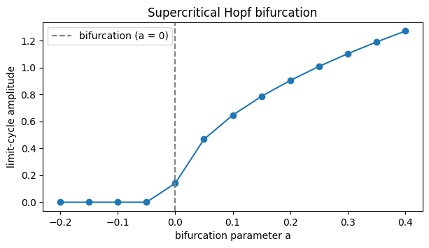
The amplitude is flat at zero while a < 0 (the unit is silent), then rises smoothly once
a crosses zero. A single number turned a quiet node into a sustained oscillator — that is a
bifurcation, and it is the reason these models are useful for studying rhythm generation.
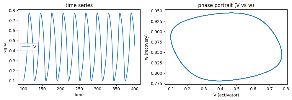
An excitable unit: FitzHugh–Nagumo phase portrait#
The FitzHughNagumoStep we met in tutorial 01 has two variables, so its
dynamics live in a 2-D phase plane (V, w). Driven steadily it settles onto a closed
loop — the limit cycle — which brainmass.viz.plot_phase_portrait() draws by plotting
one variable against the other.
fhn = brainmass.FitzHughNagumoStep(in_size=1)
r = brainmass.Simulator(fhn, dt=0.1 * u.ms).run(
    400.0 * u.ms,
    inputs=lambda i, t: (1.0,),   # steady drive -> sustained spiking
    monitors=["V", "w"],
    transient=100.0 * u.ms,
)

fig, (ax1, ax2) = plt.subplots(1, 2, figsize=(10, 3.5))
brainmass.viz.plot_timeseries(r["V"], ts=r["ts"], labels=["V"], ax=ax1)
ax1.set_title("time series")
brainmass.viz.plot_phase_portrait(r["V"][:, 0], r["w"][:, 0], ax=ax2)
ax2.set_xlabel("V (activator)")
ax2.set_ylabel("w (recovery)")
ax2.set_title("phase portrait (V vs w)")
fig.tight_layout()
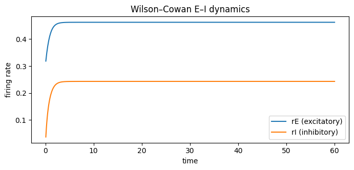
An E–I rate model: Wilson–Cowan#
The WilsonCowanStep is a physiological model: two coupled populations,
excitatory (rE) and inhibitory (rI) firing rates, with interpretable connection weights.
Depending on its parameters it can rest at a fixed point or oscillate. Here we run it from a
small perturbation and watch the two populations relax together.
wc = brainmass.WilsonCowanStep(
    in_size=1, rE_init=braintools.init.Constant(0.3)
)
r = brainmass.Simulator(wc, dt=0.1 * u.ms).run(60.0 * u.ms, monitors=["rE", "rI"])

fig, ax = plt.subplots(figsize=(8, 3.2))
brainmass.viz.plot_timeseries(r["rE"], ts=r["ts"], labels=["rE (excitatory)"], ax=ax)
brainmass.viz.plot_timeseries(r["rI"], ts=r["ts"], labels=["rI (inhibitory)"], ax=ax)
ax.set_title("Wilson–Cowan E–I dynamics")
ax.set_ylabel("firing rate");
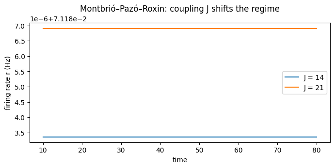
A next-generation mean-field: Montbrió–Pazó–Roxin#
The MontbrioPazoRoxinStep is an exact mean-field reduction of a network
of quadratic integrate-and-fire neurons. Its state is the population firing rate r (a
unit-aware quantity in Hz) and the mean membrane potential v. The coupling strength J
moves it between a low-rate fixed point and self-sustained oscillations.
We compare two coupling strengths and plot the firing rate over time.
fig, ax = plt.subplots(figsize=(8, 3.2))

for J in [14.0, 21.0]:
    mpr = brainmass.MontbrioPazoRoxinStep(in_size=1, J=J, eta=-5.0)
    r = brainmass.Simulator(mpr, dt=0.1 * u.ms).run(
        80.0 * u.ms, monitors=["r"], transient=10.0 * u.ms
    )
    # r['r'] is unit-aware (Hz); viz strips the unit for plotting.
    brainmass.viz.plot_timeseries(r["r"], ts=r["ts"], labels=[f"J = {J:.0f}"], ax=ax)

ax.set_title("Montbrió–Pazó–Roxin: coupling J shifts the regime")
ax.set_ylabel("firing rate r (Hz)");
What you learned#
brainmass.list_models()(and.to_table()) is your map of the model families: phenomenological, physiological, and network.A phase portrait (
plot_phase_portrait()) shows the trajectory in state space; for a 2-D model a limit cycle is a closed loop.A bifurcation is a qualitative change of behaviour as a parameter crosses a threshold — the Hopf
a, the MPR couplingJ.The same
Simulator-driven workflow applies to every model, so swapping models is cheap.
Next steps#
Noise and Stochastic Runs — real activity fluctuates; add stochastic dynamics.
Choose a Model — pick the right model for your question.
Gallery — the full model zoo, one runnable demo each.