Lorenz System

The Lorenz system is the textbook example of deterministic chaos — a three-variable flow originally derived as a truncated model of atmospheric convection:

\[\dot x = \sigma(y - x),\qquad \dot y = x(\rho - z) - y,\qquad \dot z = xy - \beta z.\]

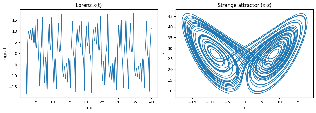
At the classic parameters \((\sigma, \rho, \beta) = (10, 28, 8/3)\) the trajectory settles onto the famous butterfly-shaped strange attractor with a positive Lyapunov exponent, so nearby trajectories diverge exponentially. In brainmass it serves as a chaotic integration / coupling test fixture. Note: use dt = 0.01 * u.ms (one natural time unit = 1 ms).

Reference: Lorenz (1963), Deterministic nonperiodic flow, Journal of the Atmospheric Sciences 20(2):130-141.

Build the model

node = brainmass.LorenzStep(in_size=1, sigma=10.0, rho=28.0)
node

LorenzStep(
  in_size=(1,),
  out_size=(1,),
  sigma=Const(
    fit=False,
    t=IdentityT(),
    reg=None,
    val=Array(10., dtype=float32)
  ),
  rho=Const(
    fit=False,
    t=IdentityT(),
    reg=None,
    val=Array(28., dtype=float32)
  ),
  beta=Const(
    fit=False,
    t=IdentityT(),
    reg=None,
    val=Array(2.6666667, dtype=float32)
  ),
  init_x=Constant(value=1.0),
  init_y=Constant(value=1.0),
  init_z=Constant(value=1.0),
  method=exp_euler
)

Run a simulation

Lorenz uses the fast dt = 0.01 * u.ms clock.

sim = brainmass.Simulator(node, dt=0.01 * u.ms)
res = sim.run(40. * u.ms, monitors=['x', 'y', 'z'], transient=2. * u.ms)
res['x'].shape

(3800, 1)

Visualize

Left: the chaotic x(t) time series. Right: the butterfly attractor in the x-z plane.

fig, axes = plt.subplots(1, 2, figsize=(11, 4))
brainmass.viz.plot_timeseries(res['x'], ts=res['ts'], ax=axes[0])
axes[0].set_title('Lorenz x(t)')
brainmass.viz.plot_phase_portrait(res['x'], res['z'], ax=axes[1])
axes[1].set_xlabel('x'); axes[1].set_ylabel('z')
axes[1].set_title('Strange attractor (x-z)')
plt.tight_layout()
plt.show()

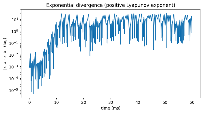
Try it: sensitive dependence on initial conditions

The hallmark of chaos: two trajectories started a hair apart diverge exponentially. We perturb the initial x by 1e-3 and plot the growing separation.

def run_from(x0):
    m = brainmass.LorenzStep(in_size=1, sigma=10.0, rho=28.0)
    brainstate.nn.init_all_states(m)
    m.x.value = m.x.value + x0
    return u.get_magnitude(
        brainmass.Simulator(m, dt=0.01 * u.ms).run(
            60. * u.ms, monitors=['x'], init_states=False)['x'])[:, 0]

a = run_from(0.0)
b = run_from(1e-3)
ts = np.arange(a.shape[0]) * 0.01
fig, ax = plt.subplots(figsize=(8, 4))
ax.semilogy(ts, np.abs(a - b) + 1e-12)
ax.set_xlabel('time (ms)'); ax.set_ylabel('|x_a - x_b|  (log)')
ax.set_title('Exponential divergence (positive Lyapunov exponent)')
plt.show()