Gradient-Free Fitting

Not every fitting problem has a usable gradient. The objective might be non-differentiable (a spike count, a discrete decision), the loss surface might be jagged, or you might be fitting a black-box metric. For these cases brainmass.Fitter exposes two gradient-free backends that search the parameter space directly:

• backend='nevergrad' – evolutionary / population-based optimisers,

• backend='scipy' – the SciPy optimiser family (gradient and gradient-free methods).

The headline of Fitter is write the objective once, swap the backend. We reuse the exact same amplitude target from Fitting with Gradients and solve it three ways, then compare the cost.

Note

The gradient-free backends search a bounded box per parameter. The box is derived automatically from a parameter’s transform when that transform defines a finite interval (e.g. SigmoidT). We use SigmoidT(0.05, 3.0) so the box is (0.05, 3.0) – no bounds need to be spelled out.

import brainmass
import brainstate
import braintools
import brainunit as u
import jax.numpy as jnp
import numpy as np
import matplotlib.pyplot as plt
from brainstate.nn import Param, SigmoidT

brainstate.environ.set(dt=0.1 * u.ms)
brainstate.random.seed(0)

An NVIDIA GPU may be present on this machine, but a CUDA-enabled jaxlib is not installed. Falling back to cpu.

The same problem as Tutorial 06

A HopfStep whose limit-cycle amplitude we match to a target generated at a known a* = 1.5. The only change from the gradient tutorial is the transform: SigmoidT(0.05, 3.0) gives the gradient-free search a finite box to explore.

def make_hopf(a, trainable=False):
    a_param = Param(a, t=SigmoidT(0.05, 3.0), fit=True) if trainable else a
    return brainmass.HopfStep(
        in_size=1, a=a_param, w=0.3,
        init_x=braintools.init.Constant(0.5),
        init_y=braintools.init.Constant(0.0),
    )

def settled_amplitude(node):
    res = brainmass.Simulator(node, dt=0.1 * u.ms).run(
        300.0 * u.ms, monitors=['x'], transient=150.0 * u.ms,
    )
    x = u.get_magnitude(res['x'])
    return jnp.sqrt(jnp.mean(x ** 2)) * jnp.sqrt(2.0)

target_amplitude = float(settled_amplitude(make_hopf(1.5)))

def loss_fn(model):                          # the SAME objective for every backend
    amp = settled_amplitude(model)
    return (amp - target_amplitude) ** 2, amp

print(f"target amplitude (true a* = 1.5): {target_amplitude:.4f}")

target amplitude (true a* = 1.5): 1.2296

Nevergrad (evolutionary search)

backend='nevergrad' runs an evolutionary optimiser over the derived box. For the gradient-free backends the optimizer argument is an options dict (or a method-name string), not a braintools.optim instance – here Differential Evolution with n_sample candidates per generation. n_steps is the number of generations, so the total number of simulations is roughly n_sample x n_steps.

node = make_hopf(0.1, trainable=True)
ng_result = brainmass.Fitter(
    node,
    {'method': 'DE', 'n_sample': 6},
    loss_fn=loss_fn,
    backend='nevergrad',
).fit(n_steps=12)

print(f"nevergrad: fitted a = {float(ng_result.best_params['a']):.4f}   (true a* = 1.5)")
print(f"           best loss = {ng_result.best_loss:.2e}")
print(f"           simulations = {len(ng_result.history)}")

nevergrad: fitted a = 1.4994   (true a* = 1.5)
           best loss = 5.84e-08
           simulations = 72

SciPy

backend='scipy' runs braintools.optim.ScipyOptimizer. Gradient methods such as L-BFGS-B differentiate through the parameter assignment; gradient-free methods such as Nelder-Mead work too. Here n_steps is the number of random restarts – a couple of restarts make the search robust to a poor starting point.

node = make_hopf(0.1, trainable=True)
sp_result = brainmass.Fitter(
    node,
    {'method': 'Nelder-Mead'},               # a derivative-free SciPy simplex method
    loss_fn=loss_fn,
    backend='scipy',
).fit(n_steps=3)

print(f"scipy: fitted a = {float(sp_result.best_params['a']):.4f}   (true a* = 1.5)")
print(f"       best loss = {sp_result.best_loss:.2e}")

/home/chaoming/miniconda3/lib/python3.13/site-packages/braintools/optim/_scipy_optimizer.py:284: RuntimeWarning: Method Nelder-Mead does not use gradient information (jac).
  results = minimize(

scipy: fitted a = 1.5000   (true a* = 1.5)
       best loss = 1.55e-11

Gradient vs gradient-free: the cost

For reference we run the gradient backend on the identical problem and tally how many forward simulations each method needed to reach a comparable loss.

# Gradient backend (as in Tutorial 06) for a head-to-head comparison.
node = make_hopf(0.1, trainable=True)
grad_result = brainmass.Fitter(
    node, braintools.optim.Adam(lr=0.1), loss_fn=loss_fn, backend='grad',
).fit(n_steps=60)

# Nevergrad reports one loss per candidate; count its simulations directly.
n_grad = len(grad_result.history)
n_nevergrad = len(ng_result.history)

print(f"{'backend':<12}{'fitted a':>10}{'best loss':>14}{'evaluations':>14}")
print("-" * 50)
print(f"{'grad':<12}{float(grad_result.best_params['a']):>10.4f}{grad_result.best_loss:>14.2e}{n_grad:>14}")
print(f"{'nevergrad':<12}{float(ng_result.best_params['a']):>10.4f}{ng_result.best_loss:>14.2e}{n_nevergrad:>14}")
print(f"{'scipy':<12}{float(sp_result.best_params['a']):>10.4f}{sp_result.best_loss:>14.2e}{'(restarts)':>14}")

backend       fitted a     best loss   evaluations
--------------------------------------------------
grad            1.5220      8.29e-05            60
nevergrad       1.4994      5.84e-08            72
scipy           1.5000      1.55e-11    (restarts)

fig, ax = plt.subplots(figsize=(7, 4))
ax.plot(grad_result.history, marker='.', lw=1.2, label=f'grad ({n_grad} evals)')
ax.plot(ng_result.history, marker='.', lw=1.0, alpha=0.8,
        label=f'nevergrad ({n_nevergrad} evals)')
ax.set_yscale('log')
ax.set_xlabel('evaluation')
ax.set_ylabel('loss')
ax.set_title('Convergence: gradient vs gradient-free')
ax.legend()
ax.grid(alpha=0.3)
plt.show()

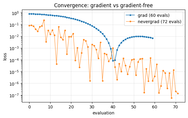
The gradient method walks straight downhill – every step is informed by the derivative, so it reaches a tiny loss in a few dozen evaluations. The evolutionary search must sample the box to discover the descent direction, so it spends many more simulations to reach a comparable loss. SciPy’s simplex sits in between.

When to use which

Situation	Backend
Differentiable objective, more than a few parameters	grad – by far the most efficient
Non-differentiable / discrete / black-box objective	nevergrad
Few parameters, well-behaved loss, want a robust local search	scipy (L-BFGS-B or Nelder-Mead)
Rugged loss with many local minima	nevergrad (population escapes local minima)

The single most important rule: if you can differentiate the objective, use grad. The whole reason brainmass models are written as differentiable JAX programs is to make that path available. Reach for gradient-free search only when the gradient is unavailable or unreliable.

Summary

• The same objective is fit by nevergrad, scipy, and grad – only the backend (and the optimizer argument’s form) changes.

• Gradient-free backends search a bounded box derived from each parameter’s transform (SigmoidT here); pass an explicit search_space for unbounded transforms.

• Gradient descent reaches the target in far fewer simulations than evolutionary search.

Next steps

• Fitting with Gradients – the gradient backend in depth.

• Training on Tasks – train a network on a cognitive task over epochs.

• Orchestration – Fitter / FitResult API and search_space derivation.