Building a Network

A whole-brain model is many neural-mass nodes wired together by a connectome: a structural-connectivity matrix of coupling weights, and (optionally) inter-region distances that become conduction delays. In this tutorial you will build one with the high-level Network class and a bundled example connectome. You will:

1. load a connectome from brainmass.datasets (no download required),

2. wire its weights and distances into a delay-coupled Network,

3. drive the whole network with the Simulator, and

4. visualise the connectivity and the multi-region activity, and compute functional connectivity.

Important

A delay-coupled Network sizes its delay buffer from the global dt at construction time, so set brainstate.environ.set(dt=...) before you build it (we do this in the import cell below).

import brainmass
import brainstate
import brainunit as u
import numpy as np
import matplotlib.pyplot as plt

# Set dt BEFORE building a delay-coupled Network (its delay buffer is sized now).
brainstate.environ.set(dt=0.1 * u.ms)

An NVIDIA GPU may be present on this machine, but a CUDA-enabled jaxlib is not installed. Falling back to cpu.

1. Load a connectome

brainmass.datasets ships small, license-clean example data so every notebook runs with no external download. load_dataset('example_connectome') returns a typed Connectome with three fields:

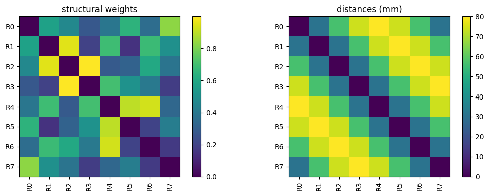
• weights — an (N, N) structural-connectivity matrix (symmetric, zero diagonal),

• distances — an (N, N) matrix of inter-region distances, unit-aware (in u.mm),

• labels — the region names.

This bundled connectome has N = 8 regions — small enough to simulate instantly and to read off the connectivity matrix by eye.

conn = brainmass.datasets.load_dataset("example_connectome")
N = conn.weights.shape[0]

print("regions:", list(conn.labels))
print("weights shape:", conn.weights.shape)
print("distances unit:", u.get_unit(conn.distances), "| max distance:", conn.distances.max())
print("zero diagonal:", bool(np.allclose(np.diag(conn.weights), 0)),
      "| symmetric:", bool(np.allclose(conn.weights, conn.weights.T)))

regions: [np.str_('R0'), np.str_('R1'), np.str_('R2'), np.str_('R3'), np.str_('R4'), np.str_('R5'), np.str_('R6'), np.str_('R7')]
weights shape: (8, 8)
distances unit: mm | max distance: 80. mm
zero diagonal: True | symmetric: True

Let us look at the connectivity matrix. brainmass.viz.plot_connectivity() draws any square matrix as a labelled heatmap — the weights on the left, the distances on the right.

fig, (ax1, ax2) = plt.subplots(1, 2, figsize=(11, 4))
brainmass.viz.plot_connectivity(conn.weights, labels=list(conn.labels), ax=ax1)
ax1.set_title("structural weights")
brainmass.viz.plot_connectivity(conn.distances, labels=list(conn.labels), ax=ax2)
ax2.set_title("distances (mm)")
fig.tight_layout()

2. Wire it into a Network

Network encapsulates the whole-brain wiring that the examples used to copy-paste: it zeros the connectivity diagonal, turns distance / speed into conduction delays, prefetches each region’s delayed state, and feeds a DiffusiveCoupling current back into the node.

We give it a bank of N HopfStep oscillators (one per region), the structural weights, the distances together with a conduction speed (so delay = distance / speed), and tell it which node state variable to couple (x) and how strongly (k).

nodes = brainmass.HopfStep(in_size=N, a=0.2, w=0.3)

net = brainmass.Network(
    nodes,
    conn=conn.weights,
    distance=conn.distances,
    speed=10.0 * u.mm / u.ms,      # conduction speed -> delays = distance / speed
    coupling="diffusive",          # k * sum_j W_ij (x_j(delayed) - x_i)
    coupled_var="x",
    k=0.5,                          # global coupling strength
)

print("network of", net.n_node, "regions, coupling:", type(net.coupling).__name__)

network of 8 regions, coupling: DiffusiveCoupling

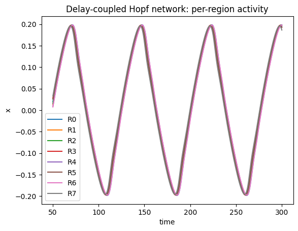
3. Drive it with the Simulator

The Simulator drives a Network exactly as it drove a single node — it does not care how many regions there are. We record the coupled state of every region each step with a callable monitor (lambda m: m.node.x.value), discarding a short transient.

sim = brainmass.Simulator(net, dt=0.1 * u.ms)
res = sim.run(
    300.0 * u.ms,
    monitors=lambda m: m.node.x.value,   # (steps, regions)
    transient=50.0 * u.ms,
)
activity = res["output"]
print("activity shape (steps, regions):", activity.shape)

ax = brainmass.viz.plot_timeseries(activity, ts=res["ts"], labels=list(conn.labels))
ax.set_title("Delay-coupled Hopf network: per-region activity")
ax.set_ylabel("x");

activity shape (steps, regions): (2500, 8)

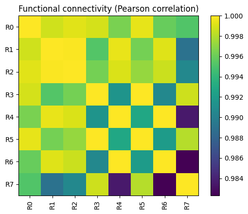
4. Functional connectivity

The structural connectivity is how the regions are wired; the functional connectivity (FC) is how correlated their activity turns out to be. brainmass.viz.plot_functional_connectivity() computes the FC matrix from a (time, region) trajectory (via braintools.metric.functional_connectivity()) and plots it. Coupling makes the regions co-vary, so the FC reflects the structure that produced it.

ax = brainmass.viz.plot_functional_connectivity(
    np.asarray(activity), labels=list(conn.labels)
)
ax.set_title("Functional connectivity (Pearson correlation)");

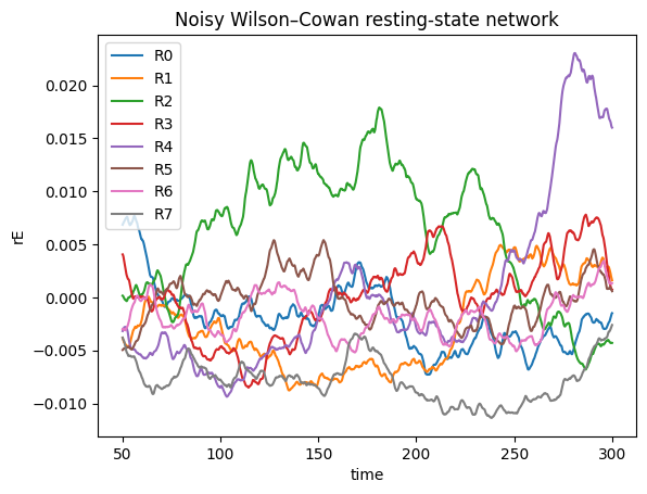
Adding noise and other node models

Everything you learned in the previous tutorials composes here. The node can be any model, and it can carry its own noise — a WilsonCowanStep bank with an OUProcess on its excitatory population gives a noisy resting-state network in a few lines. We couple the rE variable this time.

brainstate.random.seed(0)
wc_nodes = brainmass.WilsonCowanStep(
    in_size=N,
    noise_E=brainmass.OUProcess(in_size=N, sigma=0.1, tau=50.0 * u.ms),
)
wc_net = brainmass.Network(
    wc_nodes,
    conn=conn.weights,
    distance=conn.distances,
    speed=10.0 * u.mm / u.ms,
    coupled_var="rE",
    k=0.1,
)
res_wc = brainmass.Simulator(wc_net, dt=0.1 * u.ms).run(
    300.0 * u.ms, monitors=lambda m: m.node.rE.value, transient=50.0 * u.ms
)
ax = brainmass.viz.plot_timeseries(res_wc["output"], ts=res_wc["ts"], labels=list(conn.labels))
ax.set_title("Noisy Wilson–Cowan resting-state network")
ax.set_ylabel("rE");

What you learned

• brainmass.datasets provides a bundled example_connectome (weights + mm distances + labels) so networks are runnable with no download.

• Network wires a node bank into a delay-coupled whole-brain model: conn (weights), distance + speed (→ delays), coupled_var, and k.

• The Simulator drives a network exactly like a single node.

• brainmass.viz plots the connectivity, the per-region activity, and the functional connectivity.

• Any node model and any noise process composes inside a Network.

Tip

Network is the high-level builder. If you need a custom coupling rule — to wire the delayed-state prefetch and coupling kernel by hand — see Custom Coupling.

Next steps

• Forward Models — map network activity to BOLD / EEG / MEG signals.

• Fitting with Gradients — fit network parameters to data with gradients.

• Custom Coupling — build a bespoke coupling by hand.