
Custom Coupling#
Goal: choose and configure the coupling that connects regions in a brainmass
network — linear (diffusive / additive / laplacian) or nonlinear
(sigmoidal / tanh / sigmoidal_jansen_rit) — and understand when to use each.
The fastest path is the coupling= argument of brainmass.Network, which wires
the right coupling object onto a delayed connectome read for you. We use that
throughout, then peek at the underlying coupling classes for the cases where you
need direct control. See Building a Network for general
network setup.
The coupling family#
A coupling turns the connectome W and the (optionally delayed) source states
into a per-region input current C_i. brainmass ships two families:
Linear — the input is a weighted sum of source states:
|
Class |
Formula |
|---|---|---|
|
|
\(C_i = k \sum_j W_{ij}(x_j - x_i)\) |
|
|
\(C_i = k \sum_j W_{ij} x_j + b\) |
|
|
\(C_i = -k\,(L x)_i\) |
Nonlinear — a saturating function is applied either after the sum (post-nonlinearity) or to each source before it (pre-nonlinearity):
|
Class |
Formula |
When |
|---|---|---|---|
|
|
\(C_i = k\,\tanh(\mathrm{scale}\sum_j W_{ij}x_j)\) |
symmetric saturation to \(\pm k\) |
|
|
\(C_i = k\,\sigma(\mathrm{slope}(a\sum_j W_{ij}x_j + b - \mathrm{mid}))\) |
asymmetric firing-rate saturation |
|
|
\(C_i = k\sum_j W_{ij}\,\sigma_{JR}(x_j)\) |
Jansen-Rit pre-synaptic transfer |
The global strength k is TVB’s G (G ≡ k).
Build a network and swap couplings#
Set up a connectome and a node once, then change only coupling=. We use the
bundled 8-region connectome and a Hopf node; the Simulator drives the network.
Note
A delay-coupled Network sizes its delay buffers from the global dt at
construction time, so set brainstate.environ.set(dt=...) once before building
any network. The Simulator also supplies dt at run time.
conn = brainmass.datasets.load_dataset('example_connectome')
W, D = conn.weights, conn.distances
N = W.shape[0]
brainstate.environ.set(dt=0.1 * u.ms)

def run_with(coupling, **kw):
    kw.setdefault('k', 0.5)
    node = brainmass.HopfStep(in_size=N, a=0.2, w=0.3,
                              init_x=braintools.init.Constant(0.3))
    net = brainmass.Network(node, conn=W, distance=D, speed=10 * u.mm / u.ms,
                            coupling=coupling, coupled_var='x', **kw)
    res = brainmass.Simulator(net, dt=0.1 * u.ms).run(
        300 * u.ms, monitors=lambda m: m.node.x.value, transient=50 * u.ms)
    return u.get_magnitude(res['output'])

for c in ['diffusive', 'additive', 'tanh', 'sigmoidal']:
    sig = run_with(c)
    print(f"{c:12s} -> trajectory {sig.shape}, mean|x| = {np.abs(sig).mean():.3f}")
diffusive    -> trajectory (2500, 8), mean|x| = 0.117
additive     -> trajectory (2500, 8), mean|x| = 1.359
tanh         -> trajectory (2500, 8), mean|x| = 0.727
sigmoidal    -> trajectory (2500, 8), mean|x| = 0.692
Linear couplings#
Diffusive#
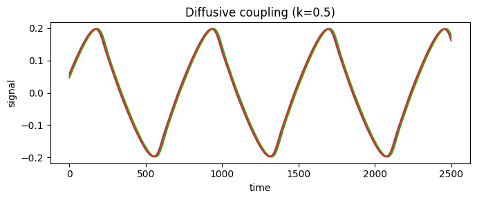
Diffusive coupling drives each node toward its neighbours’ states — the \(x_j - x_i\) difference vanishes when the network synchronizes, so it is the natural model for synchronization and the default for brain networks.
sig_diff = run_with('diffusive')
fig, ax = plt.subplots(figsize=(7, 3))
brainmass.viz.plot_timeseries(sig_diff[:, :4], ax=ax)
ax.set_title("Diffusive coupling (k=0.5)")
fig.tight_layout(); plt.show()
Additive#
Additive coupling sums neighbour inputs directly (\(\sum_j W_{ij} x_j\), no
self-term) — simpler, and the right choice when the drive is a genuine input
rather than a pull toward consensus. It also accepts a constant bias b.
Laplacian#
coupling='laplacian' expresses diffusive coupling through the graph Laplacian
\(L = D - W\). It is mathematically equivalent to diffusive coupling on a symmetric
W but lets you reuse a precomputed Laplacian; brainmass.laplacian_connectivity
builds normalized variants.
L = brainmass.laplacian_connectivity(W, normalize=None)
print("Laplacian row sums (~0):", float(jnp.abs(L.sum(axis=1)).max()))
L_sym = brainmass.laplacian_connectivity(W, normalize="sym")   # symmetric-normalized
L_rw = brainmass.laplacian_connectivity(W, normalize="rw")     # random-walk
print("normalized Laplacians:", L_sym.shape, L_rw.shape)

sig_lap = run_with('laplacian')
print("laplacian network ran:", sig_lap.shape)
Laplacian row sums (~0): 4.440892098500626e-16
normalized Laplacians: (8, 8) (8, 8)
/home/chaoming/miniconda3/lib/python3.13/site-packages/jax/_src/numpy/lax_numpy.py:5737: UserWarning: Explicitly requested dtype float64 requested in eye is not available, and will be truncated to dtype float32. To enable more dtypes, set the jax_enable_x64 configuration option or the JAX_ENABLE_X64 shell environment variable. See https://github.com/jax-ml/jax#current-gotchas for more.
  output = _eye(N, M=M, k=k, dtype=dtype)
laplacian network ran: (2500, 8)
Nonlinear couplings#
Nonlinear couplings saturate the transmitted signal, which keeps a strongly coupled network from blowing up and better matches the bounded firing rates of real neural populations.
Hyperbolic tangent (tanh) — symmetric saturation#
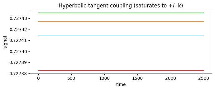
HyperbolicTangentCoupling applies tanh after the network sum, so the
coupling current saturates smoothly to \(\pm k\). Use it when you want a symmetric,
bounded version of additive coupling. Tune scale (steepness) and k (the
saturation level).
# Network uses the coupling's defaults (tanh: k forwarded, scale=2.0); for full
# control over `scale` build the coupling directly (see "Direct construction").
sig_tanh = run_with('tanh', k=0.5)
fig, ax = plt.subplots(figsize=(7, 3))
brainmass.viz.plot_timeseries(sig_tanh[:, :4], ax=ax)
ax.set_title("Hyperbolic-tangent coupling (saturates to +/- k)")
fig.tight_layout(); plt.show()
Sigmoidal — asymmetric (firing-rate) saturation#
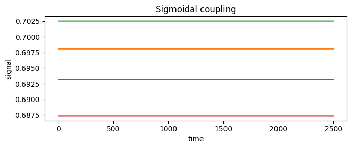
SigmoidalCoupling applies a logistic \(\sigma\) after the sum, mapping the input
to a bounded, one-sided range — the shape of a population firing-rate transfer
function. slope controls steepness, midpoint the threshold, a/b an
affine pre-scaling. At zero input the current is \(k\,\sigma(-\mathrm{slope}\cdot
\mathrm{midpoint})\).
sig_sig = run_with('sigmoidal', k=0.5)   # defaults slope=1, midpoint=0
print("sigmoidal network ran:", sig_sig.shape)
fig, ax = plt.subplots(figsize=(7, 3))
brainmass.viz.plot_timeseries(sig_sig[:, :4], ax=ax)
ax.set_title("Sigmoidal coupling")
fig.tight_layout(); plt.show()
sigmoidal network ran: (2500, 8)
Sigmoidal Jansen-Rit — pre-nonlinearity transfer#
SigmoidalJansenRitCoupling is a pre-nonlinearity: the sigmoid
\(\sigma_{JR}\) is applied to each source before the weighted sum, modelling the
presynaptic potential-to-rate transfer in the Jansen-Rit column. It is the
coupling to use for Jansen-Rit whole-brain networks, where the source is the
pyramidal input y1 - y2. Parameters cmin/cmax bound the rate, midpoint/r
shape the curve.
# Demonstrate the kernel directly on a synthetic source (pre-nonlinearity form).
src = jnp.linspace(0.0, 12.0, N)                  # presynaptic potentials
W_jr = jnp.asarray(W)
c = brainmass.sigmoidal_jansen_rit_coupling(
    src[None, :] * jnp.ones((N, N)),              # each target reads every source
    conn=W_jr, k=1.0, cmin=0.0, cmax=0.005, midpoint=6.0, r=0.56,
)
print("sigmoidal_jansen_rit output:", c.shape, " (bounded firing-rate currents)")
print("range:", float(c.min()), "->", float(c.max()))
sigmoidal_jansen_rit output: (8,)  (bounded firing-rate currents)
range: 0.004580279812216759 -> 0.01149471290409565
When wiring it into a Jansen-Rit Network, select it with
coupling='sigmoidal_jansen_rit' and coupled_var='y1' (or whatever pyramidal
observable your node exposes) — the Network plugs the delayed source read into
the coupling exactly as above.
Choosing a coupling#
diffusive— default for brain networks; models synchronization. Start here.additive— when the connectome is a genuine input current, not a consensus pull. Cheapest.laplacian— diffusive coupling via a (possibly normalized) graph Laplacian; reuse a precomputedL.tanh— when strong coupling would otherwise destabilize the network and you want a symmetric bound.sigmoidal— when the coupling should act like a population firing-rate (bounded, one-sided, thresholded).sigmoidal_jansen_rit— the canonical Jansen-Rit pre-synaptic transfer.
Tuning k:
Start around
k ~ 0.1–0.5.Increase until the network shows the connectivity / synchrony you expect.
Too high → everything synchronizes (unphysical); too low → no functional connectivity. Sweep it (see Run Parameter Sweeps).
Direct construction (advanced)#
Network is the convenient path, but you can build a coupling object directly
from prefetch references to a node’s state — useful for custom wiring (e.g.
coupling two different state variables, or asymmetric forward/backward weights).
A diffusive coupling needs a delayed (N, N) source read (each target reads every
source) plus a (N,) self read.
from brainmass import delay_index
nodes = brainmass.HopfStep(in_size=N, a=0.2, w=0.3)

delays = jnp.ones((N, N)) * (1.0 * u.ms)
idx = delay_index(N)                                    # standard (N, N) source index
x_src = nodes.prefetch_delay('x', (delays, idx),
                             init=braintools.init.Constant(0.0))   # (N, N)
x_self = nodes.prefetch('x')                            # (N,)

coupling = brainmass.DiffusiveCoupling(x_src, x_self, conn=W, k=0.5)
brainstate.nn.init_all_states(nodes)
brainstate.nn.init_all_states(coupling)
with brainstate.environ.context(i=0, t=0. * u.ms):
    current = coupling.update()                          # (N,) per-node current
print("manual diffusive current:", current.shape)
manual diffusive current: (8,)
The nonlinear classes (SigmoidalCoupling, HyperbolicTangentCoupling,
SigmoidalJansenRitCoupling) construct the same way — pass the prefetched source,
conn, and the shape parameters. Any of these parameters can be a trainable
Param for fitting (see Fitting with Gradients).
Troubleshooting#
Network explodes → lower
k, normalizeW(divide by row sums or max), or switch to a saturating (tanh/sigmoidal) coupling.No synchronization → raise
k; check for isolated nodes inW; run longer.Shape error from a coupling → diffusive coupling needs a
(N, N)source read (viaprefetch_delay) and a(N,)self read; a plainprefetch('x')for the source is too small.
Next steps#
Building a Network — full network construction.
Run Parameter Sweeps — sweep the coupling strength
k.Analyze Results (FC / FCD / spectra) — measure the FC the coupling produces.
Coupling Mechanisms — the coupling API reference.