What Is a Neural Mass Model?

A neural mass model (NMM) is a low-dimensional dynamical system that describes the average activity of a large population of neurons with a handful of state variables and ordinary differential equations (ODEs). Instead of tracking the membrane potential and spikes of every cell, an NMM tracks population-level quantities — a mean firing rate, an average synaptic current, a mean membrane potential — and how they evolve in time.

This page explains the core idea, where it sits between single-neuron models and whole-brain models, and the two flavours of NMM you will meet in brainmass. It is understanding-oriented: light on code, focused on intuition. For hands-on recipes, see the Tutorials; for the package design, see Architecture Overview.

The mean-field idea

A cortical column or brain region contains on the order of \(10^5\)–\(10^6\) neurons. Simulating each one is expensive and — for many questions about rhythms, large-scale dynamics, and neuroimaging signals — unnecessary. The mean-field approximation replaces the population by its statistics.

The intuition is the law of large numbers. If \(N\) neurons each contribute a noisy spike train, the population-averaged firing rate

\[ r(t) \;=\; \frac{1}{N}\sum_{k=1}^{N} \text{(spikes of neuron $k$ near time $t$)} \]

fluctuates far less than any single neuron and, in the large-\(N\) limit, follows a smooth, deterministic equation. A neural mass model is a closed set of ODEs for such population averages, for example a mean rate \(r\) and a mean membrane potential \(v\):

\[ \tau \,\dot r = F(r, v, \text{input}), \qquad \tau \,\dot v = G(r, v, \text{input}). \]

The functions \(F\) and \(G\) encode the population’s input–output behaviour (a sigmoidal f–I curve), its synaptic time constants, and its recurrent connectivity. The price of this compression is that you give up single-spike information; the reward is that a whole brain region becomes 1–6 numbers you can simulate, fit, and differentiate cheaply.

Populations, not single neurons

It helps to place the NMM on a ladder of abstraction:

Level	State per unit	Typical # of units for a brain	Captures
Single-neuron (Hodgkin–Huxley, LIF)	membrane potential, gating, spikes	\(10^9\)–\(10^{11}\)	individual spikes, biophysics
Neural mass / mean field	mean rate / potential (1–6 vars)	tens–hundreds (one per region)	population rhythms, regional dynamics
Neural field	activity over a continuous sheet	a field \(u(x,t)\)	spatial patterns, travelling waves

The NMM lives at the population rung. One “unit” is not a neuron — it is an entire population (a column, a region, an excitatory or inhibitory pool). This is exactly the right granularity for whole-brain modelling, where the data (EEG/MEG/fMRI) are themselves spatially coarse and reflect aggregate activity, not single cells.

A second key move is the excitatory–inhibitory (E–I) motif. Many NMMs model a region as coupled excitatory and inhibitory pools, because the push–pull between them generates oscillations (alpha, gamma) and stabilises activity. The Wilson–Cowan and Jansen–Rit models in brainmass are built from this motif.

Two flavours: phenomenological vs physiological

NMMs come in two broad styles, and brainmass ships both.

Phenomenological models aim to reproduce the qualitative dynamics — limit cycles, bistability, bifurcations — with the simplest possible equations, often a normal form. Their parameters are abstract (a bifurcation parameter, an angular frequency) rather than biophysical. They are ideal for studying what kind of dynamics a region can produce and for fast, well-conditioned fitting.

• Hopf / Stuart–Landau — the normal form of an oscillation; a single bifurcation parameter switches a region between a quiet fixed point and a self-sustained rhythm. The canonical “house” demo model.

• FitzHugh–Nagumo, Van der Pol — excitable / relaxation-oscillator dynamics.

• Kuramoto — phase-only oscillators for studying synchronisation.

Physiological (biophysical) models keep variables and parameters that map onto measurable biology — synaptic time constants, membrane capacitance, ion-channel conductances, firing-rate transfer functions — so their outputs can be compared to recordings in physical units.

• Jansen–Rit — three interacting populations producing realistic EEG-like waveforms in millivolts.

• Wilson–Cowan — coupled E and I firing rates with sigmoidal transfer.

• Wong–Wang — synaptic-gating dynamics used for fMRI/BOLD whole-brain models.

• Montbrió–Pazó–Roxin, Coombes–Byrne — next-generation / exact mean fields derived exactly from networks of quadratic-integrate-and-fire neurons, so the mean rate and potential carry the right biophysical meaning (see Why Differentiable? for why the exact derivation matters).

You can browse the full catalogue with brainmass.list_models() — let’s do that now.

import brainmass

# A curated registry of the models brainmass ships, with their category,
# number of state variables, and a one-line use case.
print(brainmass.list_models.to_table())

name                     category          #states  use_case                                 
-----------------------  ----------------  -------  -----------------------------------------
HopfStep                 phenomenological  2        Oscillation onset, rhythm generation     
VanDerPolStep            phenomenological  2        Nonlinear relaxation oscillations        
StuartLandauStep         phenomenological  2        Amplitude-controlled oscillations        
FitzHughNagumoStep       phenomenological  2        Excitability, spike generation           
ThresholdLinearStep      phenomenological  2        Fast linear E-I responses                
Generic2dOscillatorStep  phenomenological  2        Flexible planar dynamics (TVB)           
LorenzStep               phenomenological  3        Chaos, coupling test fixture             
LinearStep               phenomenological  1        Baseline node, coupling sanity checks    
WilsonCowanStep          physiological     2        E-I population firing-rate dynamics      
JansenRitStep            physiological     6        EEG generation, alpha rhythms            
WongWangStep             physiological     2        Decision making (perceptual choice)      
WongWangExcInhStep       physiological     2        Resting-state BOLD/FC, E-I balance       
MontbrioPazoRoxinStep    physiological     2        Exact QIF mean-field (theta neurons)     
CoombesByrneStep         physiological     2        Next-gen mean-field, conductance synapses
LarterBreakspearStep     physiological     3        Conductance-based limit cycles / chaos   
EpileptorStep            physiological     6        Seizure onset/offset, epilepsy           
KuramotoNetwork          network           1        Phase synchronization                    
HORNStep                 network           2        Single coupled-oscillator step           
HORNSeqLayer             network           2        Sequential HORN layer                    
HORNSeqNetwork           network           2        Multi-layer HORN sequence network        

The category column is exactly the phenomenological / physiological / network split discussed above, and n_state_vars is how many ODEs each region costs you — from a single phase variable up to the six-variable Epileptor.

Where NMMs sit in whole-brain modelling

A neural mass model is one component in a pipeline that turns anatomy into a predicted neuroimaging signal:

\[ \underbrace{\text{SC}}_{\text{structural connectivity}} \;\longrightarrow\; \underbrace{\text{NMM per region}}_{\text{local dynamics}} \;\longrightarrow\; \underbrace{\text{forward model}}_{\text{biophysics of measurement}} \;\longrightarrow\; \underbrace{\text{signal}}_{\text{BOLD / EEG / MEG}} \]

1. Structural connectivity (SC). A matrix of inter-region connection weights (from diffusion MRI tractography), optionally with a distance matrix that sets conduction delays. This is the wiring diagram.

2. A neural mass per region. Each node runs its own NMM. Regions exchange activity through the SC, usually as diffusive or additive coupling, with delays from finite axonal conduction speed. The maths and intuition of coupling live in Coupling and Delays.

3. A forward model. Neural activity is not measured directly. A hemodynamic model turns it into BOLD (fMRI), and lead-field models project dipolar source currents to EEG/MEG sensors. See From Activity to Signals.

4. The signal. The output you compare against data — and, in brainmass, the output you can backpropagate through to fit parameters.

In brainmass these four stages map onto Network (SC + coupling + delays), the model classes (the per-region NMM), the forward/observation models, and the Simulator / Fitter orchestration.

A small illustrative simulation

To make the mean-field idea concrete, here is a single region modelled as a Hopf oscillator. With its bifurcation parameter \(a > 0\) the region sustains a rhythm; its two state variables \((x, y)\) trace a limit cycle. This is the entire “model” — two ODEs standing in for a whole population of neurons.

import brainmass
import brainunit as u

# One region as a supercritical Hopf oscillator (a > 0 -> sustained rhythm).
node = brainmass.HopfStep(in_size=1, a=0.25, w=0.3)

res = brainmass.Simulator(node, dt=0.1 * u.ms).run(
    300 * u.ms,
    monitors=['x', 'y'],
    transient=50 * u.ms,
)

# Two population-level state variables, sampled over time.
print('x shape:', res['x'].shape, ' y shape:', res['y'].shape)
print('time runs from', res['ts'][0], 'to', res['ts'][-1])

x shape: (2500, 1)  y shape: (2500, 1)
time runs from 

50.1 ms to 300. ms

import matplotlib.pyplot as plt
import brainunit as u

fig, (ax1, ax2) = plt.subplots(1, 2, figsize=(10, 4))

# Left: the two state variables versus time (the population rhythm).
brainmass.viz.plot_timeseries(res['x'], ts=res['ts'], ax=ax1, labels=['x'])
brainmass.viz.plot_timeseries(res['y'], ts=res['ts'], ax=ax1, labels=['y'])
ax1.set_title('Population activity over time')

# Right: the same trajectory in state space -> a limit cycle.
brainmass.viz.plot_phase_portrait(res['x'][:, 0], res['y'][:, 0], ax=ax2)
ax2.set_title('Phase portrait (limit cycle)')

fig.tight_layout()
plt.show()

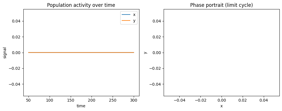
The left panel shows the population rhythm; the right shows that the two state variables settle onto a closed orbit — a limit cycle, the signature of a self-sustained oscillation. A single number, the bifurcation parameter \(a\), controls whether this cycle exists at all. That is the power of the mean-field abstraction: rich, data-relevant dynamics from a tiny, tractable system.

Key takeaways

• A neural mass model trades single-neuron detail for a handful of population-averaged ODEs per region, justified by the mean-field approximation.

• A “unit” is a population/region, not a neuron — the right granularity for whole-brain modelling and coarse neuroimaging data.

• Phenomenological models capture qualitative dynamics with abstract parameters; physiological (incl. next-generation exact) models keep biophysical meaning. brainmass ships both.

• An NMM is one stage of the whole-brain pipeline SC → NMM → forward model → signal, and in brainmass the whole pipeline is differentiable.

See also

• Why Differentiable? — why a differentiable JAX core changes how you fit and train these models.

• Architecture Overview — how the package realises the pipeline.

• Coupling and Delays — wiring regions together.

• From Activity to Signals — turning activity into BOLD / EEG / MEG.

• Tutorials — hands-on first simulations.

References

• Wilson, H. R., & Cowan, J. D. (1972). Excitatory and inhibitory interactions in localized populations of model neurons. Biophysical Journal, 12(1), 1–24.

• Jansen, B. H., & Rit, V. G. (1995). Electroencephalogram and visual evoked potential generation in a mathematical model of coupled cortical columns. Biological Cybernetics, 73(4), 357–366.

• Deco, G., Jirsa, V. K., Robinson, P. A., Breakspear, M., & Friston, K. (2008). The dynamic brain: from spiking neurons to neural masses and cortical fields. PLoS Computational Biology, 4(8), e1000092.

• Montbrió, E., Pazó, D., & Roxin, A. (2015). Macroscopic description for networks of spiking neurons. Physical Review X, 5(2), 021028.