Analyze Results (FC / FCD / spectra)

Goal: turn a simulated (or empirical) trajectory into the standard whole-brain summaries — functional connectivity (FC), FC dynamics (FCD), and power spectra — and visualize them.

brainmass does not reimplement these metrics: it surfaces braintools.metric (functional_connectivity, functional_connectivity_dynamics, power_spectral_density) and provides thin brainmass.viz plotters on top. This recipe is the post-hoc analysis half of a study; for fitting against these summaries see Compose a Custom Objective.

Produce a trajectory

We need a multi-region signal with real, oscillatory fluctuations so every summary is non-trivial. A noisy Hopf Network near its bifurcation on the bundled 8-region connectome gives spontaneous, correlated rhythms — the kind of resting-state activity FC / FCD / spectra are designed for.

conn = brainmass.datasets.load_dataset('example_connectome')
W, D = conn.weights, conn.distances
N = W.shape[0]
labels = list(conn.labels)

node = brainmass.HopfStep(
    in_size=N, a=0.1, w=0.3,           # just past the oscillation onset
    noise_x=brainmass.OUProcess(N, sigma=0.1, tau=10 * u.ms),
)
brainstate.environ.set(dt=0.1 * u.ms)
net = brainmass.Network(node, conn=W, distance=D, speed=10 * u.mm / u.ms,
                        coupling='diffusive', coupled_var='x', k=0.5)

brainstate.random.seed(0)
res = brainmass.Simulator(net, dt=0.1 * u.ms).run(
    4000 * u.ms,
    monitors=lambda m: m.node.x.value,
    transient=400 * u.ms,
    sample_every=10,             # record every 1 ms
)
signal = res['output']           # (time, regions), unit-aware
print("trajectory:", signal.shape, "  std:", round(float(u.get_magnitude(signal).std()), 4))

trajectory: (3600, 8)   std: 0.0662

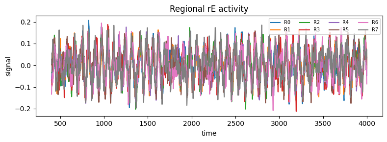
Time series

Always eyeball the raw signal first. brainmass.viz.plot_timeseries strips units and accepts the 'ts' time axis directly.

fig, ax = plt.subplots(figsize=(8, 3))
brainmass.viz.plot_timeseries(signal, ts=res['ts'], labels=labels, ax=ax)
ax.set_title('Regional rE activity')
ax.legend(fontsize=7, ncol=4, loc='upper right')
fig.tight_layout()
plt.show()

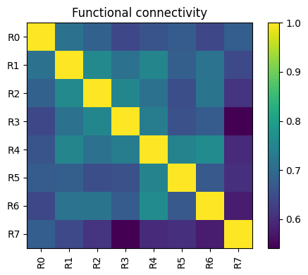
Functional connectivity (FC)

FC is the matrix of pairwise correlations between region time series — the most common static summary of coordinated activity. Compute it with braintools.metric.functional_connectivity and plot it with brainmass.viz.plot_functional_connectivity (which can also compute FC for you from a time series — pass the raw signal, no is_matrix).

sig = u.get_magnitude(signal)
fc = braintools.metric.functional_connectivity(sig)
print("FC matrix:", fc.shape)

iu = np.triu_indices(N, 1)
print("mean off-diagonal FC:", round(float(fc[iu].mean()), 3))

fig, ax = plt.subplots(figsize=(5, 4))
brainmass.viz.plot_functional_connectivity(sig, labels=labels, ax=ax)
ax.set_title('Functional connectivity')
fig.tight_layout()
plt.show()

FC matrix: (8, 8)
mean off-diagonal FC: 0.677

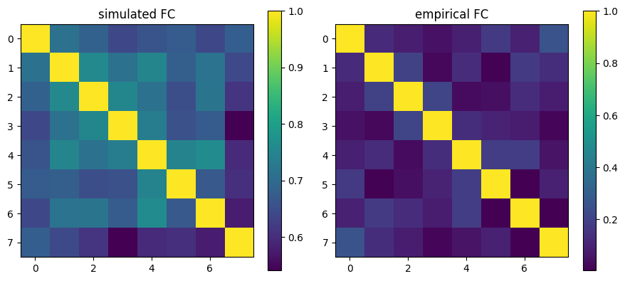
Compare simulated FC to a target

The point of FC is usually comparison to empirical data. The bundled example_signal ships a precomputed FC; score the match with an objective from brainmass.objectives (which wraps matrix_correlation).

emp = brainmass.datasets.load_dataset('example_signal')
emp_fc = emp.fc                        # (8, 8) empirical FC
score = objectives.fc_corr()(sig, emp.signal)
print("FC correlation (sim vs empirical):", round(float(score), 3))

fig, axes = plt.subplots(1, 2, figsize=(9, 4))
brainmass.viz.plot_connectivity(fc, ax=axes[0]); axes[0].set_title('simulated FC')
brainmass.viz.plot_connectivity(emp_fc, ax=axes[1]); axes[1].set_title('empirical FC')
fig.tight_layout()
plt.show()

FC correlation (sim vs empirical): 0.573

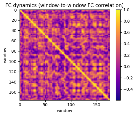
FC dynamics (FCD)

FC computed over the whole run hides non-stationarity. FCD slides a window along the signal, computes an FC per window, and correlates every pair of windowed FCs — so the FCD matrix shows how connectivity itself drifts over time. This surfaces braintools.metric.functional_connectivity_dynamics (the same metric brainmass.objectives.fcd is built on).

fcd = braintools.metric.functional_connectivity_dynamics(
    sig, window_size=100, step_size=20,   # samples (1 ms each here)
)
print("FCD matrix:", fcd.shape, "(n_windows, n_windows)")

fig, ax = plt.subplots(figsize=(5, 4))
brainmass.viz.plot_connectivity(fcd, ax=ax, cmap='plasma')
ax.set_title('FC dynamics (window-to-window FC correlation)')
ax.set_xlabel('window'); ax.set_ylabel('window')
fig.tight_layout()
plt.show()

FCD matrix: (176, 176) (n_windows, n_windows)

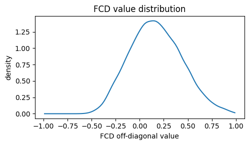
The distribution of FCD off-diagonal values is the standard FCD fitting target (a few stable states give a different distribution than a smoothly drifting one). brainmass.objectives.fcd_distribution returns it as a smooth density.

density = objectives.fcd_distribution(jnp.asarray(fcd))
midpoints = np.linspace(-0.99, 0.99, len(density))

fig, ax = plt.subplots(figsize=(5, 3))
ax.plot(midpoints, np.asarray(density))
ax.set_xlabel('FCD off-diagonal value')
ax.set_ylabel('density')
ax.set_title('FCD value distribution')
fig.tight_layout()
plt.show()

Power spectra

The frequency content tells you which rhythms the model produces. brainmass.viz.plot_power_spectrum surfaces braintools.metric.power_spectral_density for a single region; the dt you pass sets the frequency units (a Quantity is converted to ms).

fig, ax = plt.subplots(figsize=(5, 3))
for r in range(3):
    brainmass.viz.plot_power_spectrum(sig[:, r], dt=res['ts'][1] - res['ts'][0],
                                      ax=ax, label=labels[r])
ax.set_title('Power spectra (first 3 regions)')
ax.legend(fontsize=8)
fig.tight_layout()
plt.show()

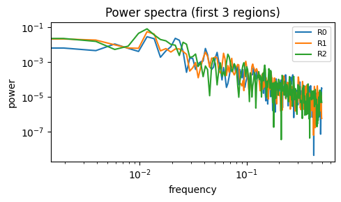
For an aggregate view, average the per-region PSDs to get the network’s mean spectrum and read off the dominant frequency.

dt_ms = float((res['ts'][1] - res['ts'][0]).to(u.ms).mantissa)
freqs, psd0 = braintools.metric.power_spectral_density(sig[:, 0], dt_ms)
psds = np.stack([
    braintools.metric.power_spectral_density(sig[:, r], dt_ms)[1]
    for r in range(N)
])
mean_psd = psds.mean(axis=0)
peak_hz = float(np.asarray(freqs)[np.argmax(mean_psd)]) * 1e3   # cycles/ms -> Hz
print("dominant network frequency:", round(peak_hz, 1), "Hz")

dominant network frequency: 11.7 Hz

Recap

Summary	Metric (braintools)	Plotter (brainmass.viz)
Time series	—	plot_timeseries
FC	functional_connectivity	plot_functional_connectivity
FCD	functional_connectivity_dynamics	plot_connectivity
Spectrum	power_spectral_density	plot_power_spectrum

These are exactly the quantities the brainmass.objectives builders score against, so the analysis you run here is the loss you would fit in Fitting with Gradients.

Next steps

• Compose a Custom Objective — fit a model to these summaries.

• Run Parameter Sweeps — sweep parameters and watch FC change.

• Forward Models — map activity to BOLD / EEG / MEG first.

• Visualization — the full visualization API.