
Choose a Model#
Goal: pick the right neural-mass model for your research question, fast.
brainmass ships ~20 models. This recipe gives you a programmatic catalogue
(brainmass.list_models), a short decision guide, and a couple of one-liners to
sanity-check a candidate before committing. For the full reference see
Neural Mass Models; to see models running, browse the
Gallery.
Browse the catalogue#
brainmass.list_models() returns one typed ModelInfo record per user-facing
model — name, category, number of state variables, and a one-line use case. It is
dependency-free and pleasant to scan in the REPL.
records = brainmass.list_models()
print(f"{len(records)} models")
print(brainmass.list_models.to_table())
20 models
name                     category          #states  use_case
-----------------------  ----------------  -------  -----------------------------------------
HopfStep                 phenomenological  2        Oscillation onset, rhythm generation
VanDerPolStep            phenomenological  2        Nonlinear relaxation oscillations
StuartLandauStep         phenomenological  2        Amplitude-controlled oscillations
FitzHughNagumoStep       phenomenological  2        Excitability, spike generation
ThresholdLinearStep      phenomenological  2        Fast linear E-I responses
Generic2dOscillatorStep  phenomenological  2        Flexible planar dynamics (TVB)
LorenzStep               phenomenological  3        Chaos, coupling test fixture
LinearStep               phenomenological  1        Baseline node, coupling sanity checks
WilsonCowanStep          physiological     2        E-I population firing-rate dynamics
JansenRitStep            physiological     6        EEG generation, alpha rhythms
WongWangStep             physiological     2        Decision making (perceptual choice)
WongWangExcInhStep       physiological     2        Resting-state BOLD/FC, E-I balance
MontbrioPazoRoxinStep    physiological     2        Exact QIF mean-field (theta neurons)
CoombesByrneStep         physiological     2        Next-gen mean-field, conductance synapses
LarterBreakspearStep     physiological     3        Conductance-based limit cycles / chaos
EpileptorStep            physiological     6        Seizure onset/offset, epilepsy
KuramotoNetwork          network           1        Phase synchronization
HORNStep                 network           2        Single coupled-oscillator step
HORNSeqLayer             network           2        Sequential HORN layer
HORNSeqNetwork           network           2        Multi-layer HORN sequence network
Each record is a NamedTuple, so you can filter it like ordinary data — for
example, “show me every physiological model with at most 3 state variables”:
cheap_physio = [
    m for m in records
    if m.category == 'physiological' and m.n_state_vars <= 3
]
for m in cheap_physio:
    print(f"{m.name:24s} {m.n_state_vars} vars  -  {m.use_case}")
WilsonCowanStep          2 vars  -  E-I population firing-rate dynamics
WongWangStep             2 vars  -  Decision making (perceptual choice)
WongWangExcInhStep       2 vars  -  Resting-state BOLD/FC, E-I balance
MontbrioPazoRoxinStep    2 vars  -  Exact QIF mean-field (theta neurons)
CoombesByrneStep         2 vars  -  Next-gen mean-field, conductance synapses
LarterBreakspearStep     3 vars  -  Conductance-based limit cycles / chaos
The three categories are:
phenomenological— generic dynamical systems (Hopf, FitzHugh-Nagumo, Stuart-Landau, …). Cheap, interpretable, great for studying bifurcations and synchronization.physiological— biophysically grounded mean-field models (Jansen-Rit, Wilson-Cowan, Wong-Wang, Montbrió-Pazó-Roxin, …). Use when you need to link to a neural mechanism or a recording modality.network— models that are a network of units (Kuramoto, the HORN family).
from collections import Counter
counts = Counter(m.category for m in records)
print(dict(counts))
{'phenomenological': 8, 'physiological': 8, 'network': 4}
A decision guide#
Walk these three axes — dynamics regime, number of variables / cost, and signal type — and the catalogue narrows quickly.
What are you studying?
├─ Generic dynamics (bifurcation, synchrony) ──► phenomenological
│   ├─ oscillation onset / rhythms ............ HopfStep, StuartLandauStep
│   ├─ excitability / spikes .................. FitzHughNagumoStep
│   ├─ phase synchronization ................... KuramotoNetwork
│   └─ a flexible planar node (TVB) ........... Generic2dOscillatorStep
│
└─ A specific neural mechanism / modality ──── physiological
    ├─ EEG / MEG, alpha rhythms .............. JansenRitStep   (6 vars)
    ├─ resting-state fMRI BOLD / FC .......... WongWangExcInhStep, WilsonCowanStep
    ├─ E-I population balance ................ WilsonCowanStep
    ├─ exact spiking mean-field .............. MontbrioPazoRoxinStep, CoombesByrneStep
    └─ seizures / epilepsy ................... EpileptorStep
Three quick rules of thumb:
Match the timescale to the data. Jansen-Rit (τ ≈ 10 ms) is right for EEG; Wong-Wang (τ ≈ 100 ms) is right for fMRI. A mismatch shows up as the wrong spectral peak.
Match the observable. EEG/MEG needs a model with an explicit membrane potential (Jansen-Rit
eeg()); BOLD needs slow synaptic dynamics (WongWangExcInhStep,WilsonCowanStep) feeding a hemodynamic model.Start cheap. Fewer state variables → faster runs and a smoother fitting landscape. Add complexity only when a simpler model demonstrably can’t fit.
Note
For resting-state BOLD use WongWangExcInhStep (the Deco-2014 excitatory /
inhibitory model with S_E/S_I states). WongWangStep is the reduced
decision-making model (S1/S2) — a different model with the same surname.
Sanity-check a candidate#
Every node model has the same contract: construct it with in_size=N, then drive
it with a brainmass.Simulator. No hand-written loop is needed — the simulator
compiles the run for you. Here is a cheap phenomenological pick (Hopf) for 90
regions.
hopf = brainmass.HopfStep(
    in_size=90,
    w=0.1,   # intrinsic angular frequency (dimensionless)
    a=0.25,  # > 0 for a stable limit cycle
)
res = brainmass.Simulator(hopf, dt=0.1 * u.ms).run(
    300 * u.ms, monitors=['x'], transient=50 * u.ms,
)
print("Hopf trace:", res['x'].shape, " (time, regions)")
Hopf trace: (2500, 90) (time, regions)
A physiological pick costs more per region — Jansen-Rit integrates 6 state
variables — but the call is identical, which is the whole point of the model
contract. Here eeg() is the derived pyramidal observable you would feed a
lead-field.
jr = brainmass.JansenRitStep(in_size=8)  # 8 cortical sources
res = brainmass.Simulator(jr, dt=0.1 * u.ms).run(
    400 * u.ms, monitors=lambda m: m.eeg(), transient=100 * u.ms,
)
print("Jansen-Rit EEG observable:", res['output'].shape)
print("n_state_vars (from catalogue):",
      next(m.n_state_vars for m in records if m.name == 'JansenRitStep'))
Jansen-Rit EEG observable: (3000, 8)
n_state_vars (from catalogue): 6
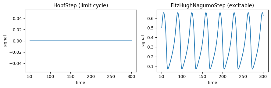
Compare candidates side by side#
Because the run API is uniform, comparing two models is just two Simulator
calls. Here a cheap oscillator (Hopf) and an excitable node (FitzHugh-Nagumo) are
each driven for the same duration; we plot one region of each.
hopf = brainmass.HopfStep(in_size=1, a=0.25, w=0.3)
fhn = brainmass.FitzHughNagumoStep(in_size=1)

r_hopf = brainmass.Simulator(hopf, dt=0.1 * u.ms).run(
    300 * u.ms, monitors=['x'], transient=50 * u.ms)
r_fhn = brainmass.Simulator(fhn, dt=0.1 * u.ms).run(
    300 * u.ms, monitors=['V'], transient=50 * u.ms,
    inputs=lambda i, t: 0.8)  # constant drive into the excitable regime

fig, axes = plt.subplots(1, 2, figsize=(9, 3))
brainmass.viz.plot_timeseries(r_hopf['x'], ts=r_hopf['ts'], ax=axes[0])
axes[0].set_title('HopfStep (limit cycle)')
brainmass.viz.plot_timeseries(r_fhn['V'], ts=r_fhn['ts'], ax=axes[1])
axes[1].set_title('FitzHughNagumoStep (excitable)')
fig.tight_layout()
plt.show()
Common pitfalls#
Reaching for a complex model too early. More parameters means a harder optimization with more local minima. Start with
HopfSteporWilsonCowanStep, validate, then add complexity.Mismatched observable. Fitting a BOLD target with a model that has no slow synaptic dynamics will never work — check the signal type axis first.
Ignoring cost. A 6-variable Jansen-Rit network is ~3× the work of a 2-variable Hopf network of the same size; for exploratory sweeps prefer the cheaper node.
Next steps#
Building a Network — wire your chosen model into a network.
Fitting with Gradients — fit its parameters.
Neural Mass Models — the full per-model reference.
Gallery — every model running end to end.