Perceptual Decision-Making with Wong-Wang

The Wong-Wang model (Wong & Wang, 2006) is the canonical reduced circuit for a two-choice perceptual decision. Two populations of neurons — one for each choice — compete through recurrent self-excitation and mutual inhibition. The competition makes the circuit bistable: from a symmetric resting state it commits to one of two high-activity attractors. A sensory evidence signal (motion coherence) biases which attractor wins, and the slow ramp of the synaptic gating variables S1/S2 is the model’s signature of evidence accumulation.

This case study demonstrates:

1. evidence accumulation — the gating variables ramping to a decision under noise,

2. bistability — symmetric (zero-evidence) trials breaking left or right at random, and

3. a psychometric sweep — choice probability vs. evidence strength.

Reference: Wong & Wang (2006), A recurrent network mechanism of time integration in perceptual decisions, J. Neurosci. 26(4):1314-1328. The model is bundled as WongWangStep — no external data needed.

Note

WongWangStep is the reduced two-variable decision model (states S1, S2; update(coherence=...)), distinct from WongWangExcInhStep, the excitatory/inhibitory mean-field model used for resting-state BOLD.

1. A single decision trial

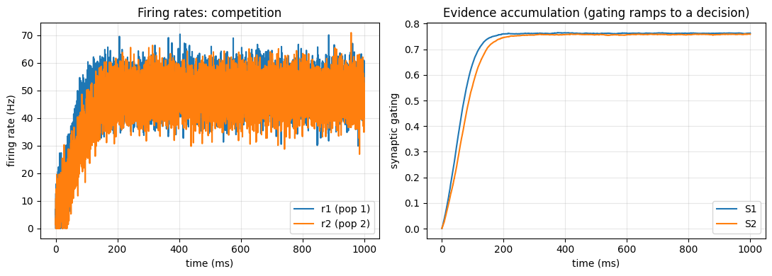
We drive the circuit with a constant rightward coherence (favoring population 1) and inject small current noise into each population so trials are stochastic. The firing rates r1, r2 start together, then one wins. The whole trial is compiled into a single brainstate.transform.for_loop() — the brainmass idiom for running a model many steps — so each trial is fast and we can run dozens of them below.

dt = 0.1 * u.ms

def run_trial(coherence, *, duration=1000.0 * u.ms, sigma=0.02 * u.nA, seed=0):
    """Run one Wong-Wang decision trial; return time, rates (r1, r2), gating (S1, S2)."""
    brainstate.random.seed(seed)
    model = brainmass.WongWangStep(
        in_size=1,
        noise_s1=brainmass.GaussianNoise(1, sigma=sigma),
        noise_s2=brainmass.GaussianNoise(1, sigma=sigma),
    )
    brainstate.nn.init_all_states(model)
    n_steps = int(duration / dt)

    def step(i):
        r1, r2 = model.update(coherence=coherence)
        return (u.get_magnitude(r1[0]), u.get_magnitude(r2[0]),
                model.S1.value[0], model.S2.value[0])

    with brainstate.environ.context(dt=dt):
        r1s, r2s, s1s, s2s = brainstate.transform.for_loop(step, np.arange(n_steps))
    ts = (np.arange(n_steps) + 1) * u.get_magnitude(dt)
    return ts, np.asarray(r1s), np.asarray(r2s), np.asarray(s1s), np.asarray(s2s)

ts, r1, r2, s1, s2 = run_trial(coherence=0.25, seed=1)
winner = 1 if s1[-1] > s2[-1] else 2
print(f"coherence = +0.25 (favors pop 1)  ->  winner: population {winner}")
print(f"final gating: S1 = {s1[-1]:.3f}, S2 = {s2[-1]:.3f}")

coherence = +0.25 (favors pop 1)  ->  winner: population 1
final gating: S1 = 0.763, S2 = 0.759

fig, (ax1, ax2) = plt.subplots(1, 2, figsize=(11, 4))
ax1.plot(ts, r1, label='r1 (pop 1)'); ax1.plot(ts, r2, label='r2 (pop 2)')
ax1.set_xlabel('time (ms)'); ax1.set_ylabel('firing rate (Hz)')
ax1.set_title('Firing rates: competition'); ax1.legend(); ax1.grid(alpha=0.3)
ax2.plot(ts, s1, label='S1'); ax2.plot(ts, s2, label='S2')
ax2.set_xlabel('time (ms)'); ax2.set_ylabel('synaptic gating')
ax2.set_title('Evidence accumulation (gating ramps to a decision)')
ax2.legend(); ax2.grid(alpha=0.3)
plt.tight_layout()
plt.show()

2. Bistability under zero evidence

With no evidence (coherence = 0) the circuit is symmetric, but noise still pushes it into one of the two attractors — and which one varies trial to trial. Running several zero-coherence trials with different noise seeds shows the spontaneous left/right split that is the hallmark of a bistable decision circuit.

fig, ax = plt.subplots(figsize=(9, 4))
n_trials = 8
choices = []
for seed in range(n_trials):
    t, _, _, s1_t, s2_t = run_trial(coherence=0.0, seed=seed)
    choice = 1 if s1_t[-1] > s2_t[-1] else 2
    choices.append(choice)
    color = 'tab:blue' if choice == 1 else 'tab:red'
    ax.plot(t, s1_t - s2_t, color=color, alpha=0.7)
ax.axhline(0, color='grey', lw=1)
ax.set_xlabel('time (ms)'); ax.set_ylabel('S1 - S2  (decision variable)')
ax.set_title(f'Zero-evidence bistability: {choices.count(1)} chose pop 1, '
             f'{choices.count(2)} chose pop 2')
plt.tight_layout()
plt.show()
print("per-trial choices (zero coherence):", choices)

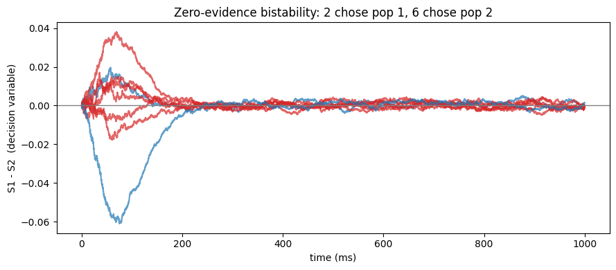
per-trial choices (zero coherence): [1, 2, 2, 2, 2, 2, 2, 1]

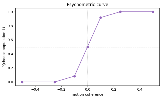
3. Psychometric curve

Sweeping the evidence strength and measuring how often population 1 wins traces a psychometric curve: chance (50%) at zero coherence, rising toward certainty as the evidence grows. We average several noisy trials per coherence level.

coherences = [-0.5, -0.25, -0.1, 0.0, 0.1, 0.25, 0.5]
n_rep = 12
p_choose_1 = []
for c in coherences:
    wins = 0
    for seed in range(n_rep):
        _, _, _, s1_t, s2_t = run_trial(coherence=c, seed=seed, duration=800.0 * u.ms)
        wins += int(s1_t[-1] > s2_t[-1])
    p_choose_1.append(wins / n_rep)
    print(f"coherence = {c:+.2f}  ->  P(choose pop 1) = {wins / n_rep:.2f}")

fig, ax = plt.subplots(figsize=(6.5, 4))
ax.plot(coherences, p_choose_1, 'o-', color='tab:purple')
ax.axhline(0.5, color='grey', ls='--', lw=1)
ax.axvline(0.0, color='grey', ls=':', lw=1)
ax.set_xlabel('motion coherence'); ax.set_ylabel('P(choose population 1)')
ax.set_ylim(-0.05, 1.05); ax.set_title('Psychometric curve')
plt.tight_layout()
plt.show()

coherence = -0.50  ->  P(choose pop 1) = 0.00

coherence = -0.25  ->  P(choose pop 1) = 0.00

coherence = -0.10  ->  P(choose pop 1) = 0.08

coherence = +0.00  ->  P(choose pop 1) = 0.50

coherence = +0.10  ->  P(choose pop 1) = 0.92

coherence = +0.25  ->  P(choose pop 1) = 1.00

coherence = +0.50  ->  P(choose pop 1) = 1.00

Summary

The Wong-Wang circuit reproduces the core phenomena of two-choice perceptual decisions:

• evidence accumulation — the synaptic gating variables S1/S2 ramp up and one wins,

• bistability — under zero evidence, noise alone breaks the symmetry left or right, and

• a psychometric curve — choice probability rises smoothly with evidence strength.

WongWangStep exposes the rates via update(coherence=...) and the gating state via model.S1 / model.S2. A constant scalar drive like coherence is passed directly to update; the noise injected through noise_s1/noise_s2 is what makes individual trials stochastic. This single-circuit model is the decision-making node you would embed in a larger network to study distributed choice.