Quickstart

This is the 10-minute tour of brainmass. By the end you will have, using only the high-level API:

1. picked a model and run it through the Simulator,

2. plotted the result with brainmass.viz,

3. added noise in a single line,

4. wired two regions into a delay-coupled Network from a bundled connectome, and

5. fit a parameter by gradient descent with the Fitter against a bundled signal.

No hand-written integration loops — the Simulator/Network/Fitter objects own the brainstate.transform machinery so you focus on the model.

Note

The integration time step dt is a unit-aware quantity (0.1 * u.ms), passed to the Simulator — it is not a model argument. Quantities flow through brainmass via brainunit, so u.ms, u.mm, … keep your numbers physically meaningful.

import brainmass
import braintools
import brainstate
import brainunit as u
import jax.numpy as jnp
import numpy as np
from brainstate.nn import Param

# `dt` is a global, set once through the environment. The Simulator also takes an
# explicit dt= below; setting it here lets delay-buffer sizing work when we build a
# Network (its conduction delays are measured in dt-steps at construction time).
brainstate.environ.set(dt=0.1 * u.ms)

brainmass.__version__

An NVIDIA GPU may be present on this machine, but a CUDA-enabled jaxlib is not installed. Falling back to cpu.

'0.0.6'

1. Pick a model and run it

A brainmass model is a *Step object — one update step of a neural-mass equation, sized for in_size regions. We pick the HopfStep oscillator in its limit-cycle regime (a > 0) and hand it to a Simulator. One .run(duration, monitors=...) call sets dt, initialises the state, steps the model, and returns the stacked trajectories as a plain dict (plus a 'ts' time axis).

node = brainmass.HopfStep(in_size=1, a=0.25, w=0.3)

sim = brainmass.Simulator(node, dt=0.1 * u.ms)
res = sim.run(200.0 * u.ms, monitors=["x", "y"], transient=20.0 * u.ms)

print("recorded keys:", list(res))
print("x trajectory shape (steps, regions):", res["x"].shape)
print("time axis:", res["ts"][:3], "...", res["ts"][-1])

recorded keys: ['x', 'y', 'ts']
x trajectory shape (steps, regions): (1800, 1)
time axis: [20.1 20.2 20.3] ms ... 200. ms

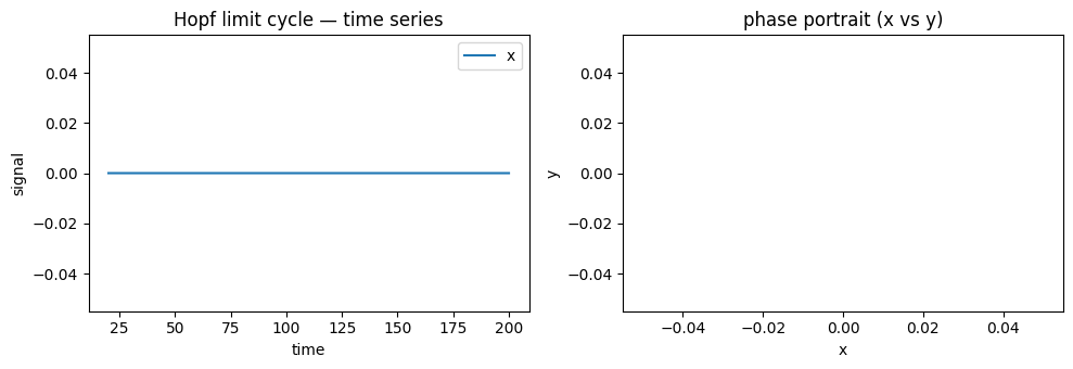
2. Plot it with brainmass.viz

brainmass.viz collects thin, matplotlib-based helpers (install the [viz] extra). plot_timeseries() takes the trajectory and the time axis directly; plot_phase_portrait() plots one state variable against another, which for a Hopf node traces out its circular limit cycle.

import matplotlib.pyplot as plt

fig, (ax1, ax2) = plt.subplots(1, 2, figsize=(10, 3.5))

brainmass.viz.plot_timeseries(res["x"], ts=res["ts"], labels=["x"], ax=ax1)
ax1.set_title("Hopf limit cycle — time series")

brainmass.viz.plot_phase_portrait(res["x"][:, 0], res["y"][:, 0], ax=ax2)
ax2.set_title("phase portrait (x vs y)")

fig.tight_layout()

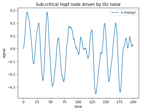
3. Add noise in one line

Real activity fluctuates. Attach an Ornstein–Uhlenbeck process (OUProcess) to a state component when you build the model — the noise is added automatically inside update(), and the Simulator call is unchanged. Here we drop the node below the bifurcation (a < 0, a stable focus) so the dynamics are noise driven rather than a clean limit cycle.

noisy = brainmass.HopfStep(
    in_size=1, a=-0.05, w=0.3,
    noise_x=brainmass.OUProcess(in_size=1, sigma=0.1, tau=20.0 * u.ms),  # <- one line
)

res_noisy = brainmass.Simulator(noisy, dt=0.1 * u.ms).run(200.0 * u.ms, monitors=["x"])

ax = brainmass.viz.plot_timeseries(res_noisy["x"], ts=res_noisy["ts"], labels=["x (noisy)"])
ax.set_title("Sub-critical Hopf node driven by OU noise");

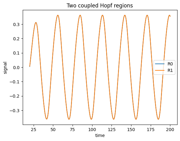
4. A two-region network (with a bundled connectome)

brainmass.datasets ships small, license-clean example data so every notebook runs with no download. load_dataset('example_connectome') returns a typed Connectome with structural weights and unit-aware distances (in u.mm).

We take the first two regions and hand them to a Network. The network zeros the self-connections, turns distance / speed into conduction delays, and feeds a diffusive coupling current back into the node — the same wiring you would otherwise write by hand. The Simulator then drives the whole network exactly as it drove the single node.

conn = brainmass.datasets.load_dataset("example_connectome")
print("connectome:", conn.weights.shape, "regions:", list(conn.labels))

# Use the first two regions as a minimal 2-node network.
W = conn.weights[:2, :2]
D = conn.distances[:2, :2]

two_nodes = brainmass.HopfStep(in_size=2, a=0.2, w=0.3)
net = brainmass.Network(
    two_nodes,
    conn=W,
    distance=D,
    speed=10.0 * u.mm / u.ms,   # delays = distance / speed
    coupling="diffusive",
    coupled_var="x",
    k=0.5,                       # global coupling strength
)

res_net = brainmass.Simulator(net, dt=0.1 * u.ms).run(
    200.0 * u.ms,
    monitors=lambda m: m.node.x.value,   # read the coupled node state each step
    transient=20.0 * u.ms,
)
print("network output shape (steps, regions):", res_net["output"].shape)

ax = brainmass.viz.plot_timeseries(
    res_net["output"], ts=res_net["ts"], labels=list(conn.labels[:2])
)
ax.set_title("Two coupled Hopf regions");

connectome: (8, 8) regions: [np.str_('R0'), np.str_('R1'), np.str_('R2'), np.str_('R3'), np.str_('R4'), np.str_('R5'), np.str_('R6'), np.str_('R7')]

network output shape (steps, regions): (1800, 2)

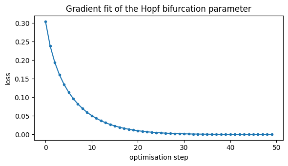
5. Fit a parameter by gradient descent

Here is brainmass’s headline capability: because the whole simulation is differentiable, you can backprop through the ODE solve and fit parameters with gradients instead of grid or evolutionary search.

We use the bundled example_signal dataset as the target. A HopfStep in its limit cycle settles at an amplitude ~sqrt(a / beta), so the bifurcation parameter a controls how big the oscillation is. We mark a trainable with Param(..., fit=True), start it too small, and let the Fitter (gradient backend) drive the simulated oscillation’s amplitude to match the data.

# Target: the RMS amplitude of region 0 of the bundled example signal.
sig = brainmass.datasets.load_dataset("example_signal")
target0 = sig.signal[:, 0]
target_amp = jnp.asarray(float(np.sqrt(np.mean((target0 - target0.mean()) ** 2))))
print("target amplitude from example_signal:", round(float(target_amp), 4))

# Model with ONE trainable parameter: the Hopf bifurcation parameter `a`.
model = brainmass.HopfStep(
    in_size=1,
    a=Param(0.05, fit=True),   # <- the single knob the Fitter will tune
    w=0.3, beta=1.0,
    init_x=braintools.init.Constant(0.5),
)


def loss_fn(m):
    """Run the model and compare its settled amplitude to the target."""
    x = brainmass.Simulator(m, dt=0.1 * u.ms).run(
        300.0 * u.ms, monitors=["x"], transient=150.0 * u.ms
    )["x"][:, 0]
    amp = jnp.sqrt(jnp.mean((x - jnp.mean(x)) ** 2))
    return (amp - target_amp) ** 2, amp


fitter = brainmass.Fitter(model, braintools.optim.Adam(lr=0.05), loss_fn=loss_fn)
result = fitter.fit(n_steps=50)

print(result)
print(f"a:        0.05  ->  {float(result.best_params['a']):.4f}")
print(f"loss:  {result.history[0]:.4f}  ->  {result.best_loss:.5f}")
print(f"amplitude matched: {float(result.prediction):.4f}  (target {float(target_amp):.4f})")

target amplitude from example_signal: 0.7152

FitResult(backend='grad', best_loss=3.10454e-07, n_steps=50, params=[a])
a:        0.05  ->  1.0262
loss:  0.3042  ->  0.00000
amplitude matched: 0.7157  (target 0.7152)

The loss curve shows the gradient optimiser converging in a few dozen steps — no parameter sweep required.

fig, ax = plt.subplots(figsize=(6, 3.5))
ax.plot(result.history, marker=".")
ax.set_xlabel("optimisation step")
ax.set_ylabel("loss")
ax.set_title("Gradient fit of the Hopf bifurcation parameter")
fig.tight_layout()

Where to go next

You have run, visualised, perturbed, coupled, and fit a model — all through the high-level API. To go deeper:

• Key Concepts — the mental model behind *Step models, Simulator, Network, Fitter and units.

• The fitting story is expanded across tutorials 06 (gradients), 07 (gradient-free) and 08 (training on tasks).

• Choose a Model — browse every model with brainmass.list_models().

• Building a Network — full whole-brain networks.

See also

• Orchestration — Simulator / Network / Fitter API.

• Datasets and Visualization — the bundled data and plotting helpers.

• Neural Mass Models — the full model reference.