Stuart-Landau Oscillator

The Stuart-Landau oscillator is the normal form of a system near a Hopf bifurcation, expressed in Cartesian coordinates as

\[\dot x = (a - x^2 - y^2)\,x - \omega\,y,\qquad \dot y = (a - x^2 - y^2)\,y + \omega\,x.\]

It is mathematically identical to the Hopf normal form: the parameter \(a\) sets the amplitude of the limit cycle (\(\sqrt{a}\)) and \(\omega\) sets the angular frequency. Networks of Stuart-Landau oscillators are widely used to model metastable synchronization in resting-state brain activity.

Reference: Kuramoto (1984), Chemical Oscillations, Waves, and Turbulence, Springer.

Build the model

node = brainmass.StuartLandauStep(in_size=1, a=0.25, w=0.5)
node

StuartLandauStep(
  in_size=(1,),
  out_size=(1,),
  init_x=Uniform(low=0, high=0.05),
  init_y=Uniform(low=0, high=0.05),
  method=exp_euler,
  a=Const(
    fit=False,
    t=IdentityT(),
    reg=None,
    val=Array(0.25, dtype=float32)
  ),
  w=Const(
    fit=False,
    t=IdentityT(),
    reg=None,
    val=Array(0.5, dtype=float32)
  )
)

Run a simulation

sim = brainmass.Simulator(node, dt=0.1 * u.ms)
res = sim.run(200. * u.ms, monitors=['x', 'y'], transient=20. * u.ms)
res['x'].shape

(1800, 1)

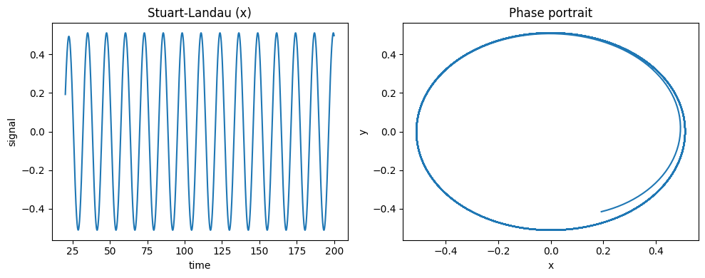
Visualize

fig, axes = plt.subplots(1, 2, figsize=(10, 4))
brainmass.viz.plot_timeseries(res['x'], ts=res['ts'], ax=axes[0])
axes[0].set_title('Stuart-Landau (x)')
brainmass.viz.plot_phase_portrait(res['x'], res['y'], ax=axes[1])
axes[1].set_title('Phase portrait')
plt.tight_layout()
plt.show()

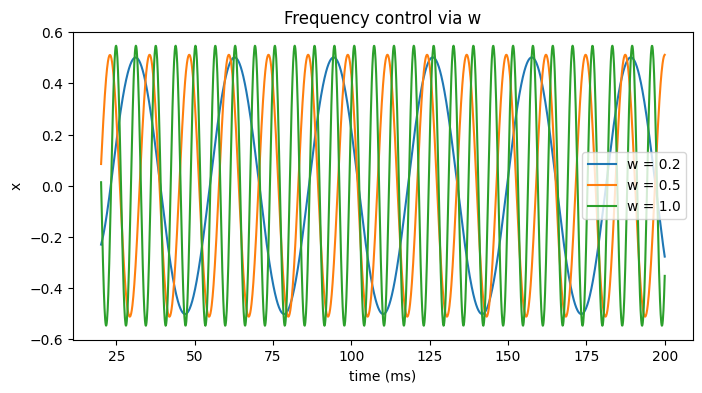
Try it: vary the intrinsic frequency w

The amplitude is fixed by a, but w sets how fast the node cycles. Higher w packs more periods into the same window.

fig, ax = plt.subplots(figsize=(8, 4))
for w in [0.2, 0.5, 1.0]:
    m = brainmass.StuartLandauStep(in_size=1, a=0.25, w=w)
    r = brainmass.Simulator(m, dt=0.1 * u.ms).run(
        200. * u.ms, monitors=['x'], transient=20. * u.ms)
    ax.plot(u.get_magnitude(r['ts']), u.get_magnitude(r['x'])[:, 0], label=f'w = {w}')
ax.set_xlabel('time (ms)'); ax.set_ylabel('x'); ax.legend()
ax.set_title('Frequency control via w')
plt.show()