Fitting with Gradients

This is what makes brainmass different. Because every model is a differentiable JAX program, you can backpropagate through the entire simulation – the ODE solve, the coupling, the forward model – and use the gradient of a loss to update model parameters. No finite differences, no black-box search: the optimiser knows exactly which way to move every parameter.

In this tutorial you will fit a model parameter to a target observation by gradient descent with brainmass.Fitter (backend='grad'). You will see:

1. a brainstate.nn.Param marked fit=True to select what is trainable,

2. a predict that runs a Simulator and reduces it to a scalar summary,

3. the gradient flowing from that scalar back through the solve to the parameter,

4. a loss curve that drops to near-zero in a few dozen evaluations.

Important

For an oscillatory model, fit a scalar summary of the trajectory (amplitude, a spectral feature, or functional connectivity) – not the raw time series with a point-by-point RMSE. Two limit cycles with the same shape but a different phase have a large pointwise RMSE, so that loss is phase-degenerate and its gradient is uninformative. We fit the settled amplitude here.

import brainmass
import brainstate
import braintools
import brainunit as u
import jax.numpy as jnp
import numpy as np
import matplotlib.pyplot as plt
from brainstate.nn import Param, SoftplusT

brainstate.environ.set(dt=0.1 * u.ms)
brainstate.random.seed(0)

An NVIDIA GPU may be present on this machine, but a CUDA-enabled jaxlib is not installed. Falling back to cpu.

The model and the scalar summary

We use a supercritical HopfStep oscillator. Above its bifurcation it settles onto a limit cycle whose radius grows with the bifurcation parameter a (for the normal form, amplitude scales as \(\sqrt{a}\)). We give it a small non-zero initial condition so the trajectory spirals out to that limit cycle, then measure the settled RMS amplitude after discarding the transient.

The summary – a single number per simulation – is what we will match to data.

def make_hopf(a, trainable=False):
    # When trainable, `a` is a bounded Param (fit=True selects it for optimisation).
    a_param = Param(a, t=SoftplusT(0.0), fit=True) if trainable else a
    return brainmass.HopfStep(
        in_size=1, a=a_param, w=0.3,
        init_x=braintools.init.Constant(0.5),   # kick off the spiral toward the limit cycle
        init_y=braintools.init.Constant(0.0),
    )

def settled_amplitude(node):
    '''Run the Simulator and reduce the trajectory to one scalar: the limit-cycle amplitude.'''
    res = brainmass.Simulator(node, dt=0.1 * u.ms).run(
        300.0 * u.ms, monitors=['x'], transient=150.0 * u.ms,
    )
    x = u.get_magnitude(res['x'])                # strip the mV-style unit before reducing
    return jnp.sqrt(jnp.mean(x ** 2)) * jnp.sqrt(2.0)   # RMS -> sinusoid amplitude

# The amplitude is a smooth, monotone function of `a` -- a well-conditioned target.
for a in [0.25, 1.0, 2.0]:
    print(f"a = {a:<4}  ->  amplitude = {float(settled_amplitude(make_hopf(a))):.3f}")

a = 0.25  ->  amplitude = 0.502
a = 1.0   ->  amplitude = 1.001
a = 2.0   ->  amplitude = 1.430

The target

In a real study the target comes from data. Here we synthesise it by running the model at a known “true” parameter a* = 1.5 and recording its amplitude – so we can check that the fit recovers it.

target_amplitude = float(settled_amplitude(make_hopf(1.5)))
print(f"target amplitude (true a* = 1.5): {target_amplitude:.4f}")

target amplitude (true a* = 1.5): 1.2296

Fit by backprop through the solve

Now the centrepiece. We start far from the truth (a = 0.1) and let Fitter minimise the squared error between the simulated amplitude and the target.

The grad backend does exactly the canonical loop: it collects the model’s trainable ParamState weights, evaluates the loss, and calls brainstate.transform.grad(...) – which differentiates through the Simulator.run for_loop – then steps the optax optimiser. We pass a loss_fn(model) -> (loss, aux) so we own the scalar reduction; the aux (the amplitude) is carried along for inspection.

node = make_hopf(0.1, trainable=True)
print("trainable parameters:", list(node.states(brainstate.ParamState).keys()))

def loss_fn(model):
    amp = settled_amplitude(model)
    loss = (amp - target_amplitude) ** 2
    return loss, amp                      # aux = current amplitude

fitter = brainmass.Fitter(
    node,
    braintools.optim.Adam(lr=0.1),        # grad backend takes a braintools.optim optimiser
    loss_fn=loss_fn,
    backend='grad',
)
result = fitter.fit(n_steps=60, verbose=False)

print(f"fitted a   : {float(result.best_params['a']):.4f}   (true a* = 1.5)")
print(f"best loss  : {result.best_loss:.2e}")
print(f"loss drop  : {result.history[0]:.4f}  ->  {result.best_loss:.2e}")
print(f"evaluations: {len(result.history)}")

trainable parameters: [('a', 'val')]

fitted a   : 1.5471   (true a* = 1.5)
best loss  : 3.37e-05
loss drop  : 0.8262  ->  3.37e-05
evaluations: 60

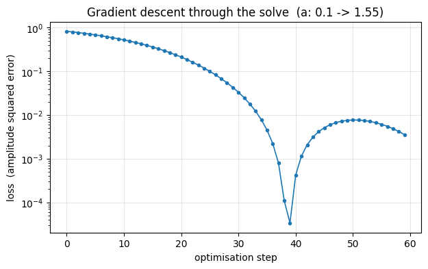
The fit recovers a* ~ 1.5 and the loss collapses by several orders of magnitude. Plotting the full loss history shows the characteristic smooth descent of a gradient method – each step moves downhill, because the gradient told it which way that is.

fig, ax = plt.subplots(figsize=(7, 4))
ax.plot(result.history, marker='.', lw=1.2)
ax.set_yscale('log')
ax.set_xlabel('optimisation step')
ax.set_ylabel('loss  (amplitude squared error)')
ax.set_title(f"Gradient descent through the solve  (a: 0.1 -> {float(result.best_params['a']):.2f})")
ax.grid(alpha=0.3)
plt.show()

Confirming the gradient is real

To make the differentiability concrete, take the gradient of the loss with respect to a directly with brainstate.transform.grad() and compare it to a finite-difference estimate. We use a plain (untransformed) Param here so autodiff and finite differences live in the same space: with a transform like SoftplusT, autodiff returns the gradient in the optimiser’s unconstrained space, which differs from a physical-space finite difference by the transform’s Jacobian (correct, but not directly comparable). With no transform they agree to several digits – the gradient that drove the fit above genuinely flows back through the entire Simulator rollout.

from brainstate.nn import Param as _Param

def loss_at(a_value):
    # Plain trainable param (no transform): unconstrained space == physical space.
    n = brainmass.HopfStep(in_size=1, a=_Param(a_value, fit=True), w=0.3,
                           init_x=braintools.init.Constant(0.5),
                           init_y=braintools.init.Constant(0.0))
    weights = n.states(brainstate.ParamState)
    (key,) = weights.keys()                       # the single trainable weight ('a', 'val')
    grad_fn = brainstate.transform.grad(
        lambda: (settled_amplitude(n) - target_amplitude) ** 2,
        weights, return_value=True,
    )
    grads, loss = grad_fn()
    return float(loss), float(grads[key])

a0 = 0.8
loss0, autodiff_grad = loss_at(a0)
eps = 1e-3
fd_grad = (loss_at(a0 + eps)[0] - loss_at(a0 - eps)[0]) / (2 * eps)
print(f"autodiff d(loss)/da  = {autodiff_grad:+.5f}")
print(f"finite-difference    = {fd_grad:+.5f}")

autodiff d(loss)/da  = -0.36418
finite-difference    = -0.36414

Selecting trainables and composing objectives

Two pieces generalise this to richer problems.

Param(fit=True) selects what is trainable. Only parameters wrapped in a Param with fit=True become ParamState weights; everything else is held fixed. A transform such as SoftplusT keeps the parameter in a valid range (here a > 0) while the optimiser works in unconstrained space.

brainmass.objectives composes losses. When you fit to a signal rather than a hand-written scalar, build the loss from the objective library – e.g. match functional connectivity with fc_corr(), or combine several terms with combine(). The example below fits a coupling gain so a 3-region Hopf network reproduces a target FC, using fc_corr(as_loss=True) (which returns 1 - corr, so minimising it maximises the correlation).

# A 3-region driven network whose FC depends on a trainable coupling gain k.
W = jnp.asarray([[0.0, 0.8, 0.2],
                 [0.8, 0.0, 0.5],
                 [0.2, 0.5, 0.0]])

def make_net(k_value, trainable=False):
    k = Param(k_value, t=SoftplusT(0.0), fit=True) if trainable else k_value
    n = brainmass.HopfStep(in_size=3, a=0.5, w=0.3,
                           noise_x=brainmass.OUProcess(3, sigma=0.3, tau=10.0 * u.ms))
    return brainmass.Network(n, conn=W, coupling='diffusive', coupled_var='x', k=k)

def predict_fc(net):
    res = brainmass.Simulator(net, dt=0.1 * u.ms).run(
        400.0 * u.ms, monitors=lambda m: m.node.x.value, transient=100.0 * u.ms,
    )
    return res['output']                          # (T, 3) time series -> FC computed by objective

# Target FC from a known coupling k* = 1.0.
brainstate.random.seed(1)
target_fc = predict_fc(make_net(1.0))

fc_loss = brainmass.objectives.fc_corr(as_loss=True)   # 1 - corr(FC_pred, FC_target)

brainstate.random.seed(1)
net = make_net(0.1, trainable=True)
fc_fitter = brainmass.Fitter(
    net, braintools.optim.Adam(lr=0.2),
    predict=predict_fc, objective=fc_loss, backend='grad',
)
fc_result = fc_fitter.fit(target=target_fc, n_steps=60)
print(f"fitted k  : {float(fc_result.best_params['coupling.k']):.3f}   (true k* = 1.0)")
print(f"FC loss   : {fc_result.history[0]:.3f}  ->  {fc_result.best_loss:.3f}")

fitted k  : 1.183   (true k* = 1.0)
FC loss   : 0.158  ->  0.000

Why gradients

The fit above converged in a few dozen forward simulations, and every one of those steps was informed by the gradient – the optimiser never had to guess a direction. That efficiency is the whole point of a differentiable simulator: for problems with more than a handful of parameters (whole-brain coupling matrices, lead-field heads, task-trained networks), gradient-based fitting is the only thing that scales.

But gradients are not always available – a non-differentiable objective, a discrete choice, a black-box metric. The next tutorial fits the same amplitude target with gradient-free search and contrasts the cost.

Summary

• brainmass models are differentiable, so Fitter with backend='grad' backpropagates through the Simulator solve.

• Mark trainables with Param(..., fit=True); reduce the trajectory to a scalar summary (amplitude / FC / spectrum), never a phase-sensitive pointwise RMSE.

• The loss curve drops smoothly; autodiff and finite-difference gradients agree.

• Compose richer losses from brainmass.objectives.

Next steps

• Gradient-Free Fitting – the same fit without gradients, and when to prefer it.

• Training on Tasks – train a network on a cognitive task over epochs.

• Orchestration – Fitter / FitResult API.