Building a Data-Driven Workflow

This is the extension playbook for data-driven modeling in brainmass: the stable contract you build a custom, fittable model against. Every piece below is a public API the rest of the ecosystem – and future tooling like the deferred Trainer (see the final section) – composes with.

We will go end to end:

1. Expose trainable parameters on a custom model with Param(value, fit=True).

2. Write a loss as a small objectives-style callable(prediction, target).

3. Fit it two ways: with the high-level brainmass.Fitter, and with a hand-written training loop over braintools.optim + brainstate.transform.grad.

4. Batch the search with vmap.

The data-driven layer is the center of gravity of brainmass (see Data-Driven Modeling). Read Creating Custom Models first for the model contract itself; this guide is about making a model learnable.

1. A model with trainable parameters

A trainable parameter is just a brainstate.nn.Param with fit=True. That wraps the value in a ParamState (a leaf the optimizers see); a plain float or Param.init(float) stays a non-trainable Const. The model is otherwise an ordinary brainstate.nn.Dynamics (see Creating Custom Models).

Two rules make a parameter gradient-friendly (learned the hard way across the fitting tutorials):

• Make the trainable dimensionless. A mV-valued Param crashes the best-parameter snapshot inside Fitter (jnp.asarray refuses a unit-carrying value). Keep the knob a plain scalar; let units live on the states.

• Fit a scalar summary, not a raw oscillatory trace. Point-by-point time-series RMSE of a limit cycle is phase-degenerate and the gradient collapses. A steady state, an amplitude, an FC value, or a spectral peak is well-conditioned.

Here is a one-population leaky-rate model whose input gain g is trainable:

class GainPopulation(brainstate.nn.Dynamics):
    """Leaky firing-rate population with a trainable input gain ``g``.

    dr/dt = (-r + g * tanh(input)) / tau
    """

    def __init__(self, in_size, g=1.0, tau=10. * u.ms):
        super().__init__(in_size)
        self.tau = tau
        # fit=True -> a trainable ParamState; a dimensionless scalar knob.
        self.g = Param(g, fit=True)

    def init_state(self, batch_size=None):
        self.r = brainstate.HiddenState(
            braintools.init.param(braintools.init.Constant(0.0),
                                  self.varshape, batch_size)
        )

    def update(self, inp=0.0):
        r = self.r.value
        dr = (-r + self.g.value() * jnp.tanh(inp)) / self.tau
        self.r.value = r + dr * brainstate.environ.get_dt()
        return self.r.value


model = GainPopulation(1, g=0.5)
brainstate.nn.init_all_states(model)
# The trainable leaves the optimizers will see:
list(model.states(brainstate.ParamState).keys())

[('g', 'val')]

states(ParamState) returns the trainable leaves keyed by tuple paths (('g', 'val')). Keep this in mind: a raw brainstate.transform.grad returns gradients keyed by exactly these tuples, whereas FitResult.best_params uses the dotted form ('g', or 'node.g' for a nested model). Same parameter, two key conventions.

2. A loss as a composable objective

An objective is a builder that returns a small callable(prediction, target) -> scalar, jit/grad/vmap-safe and unit-aware. This is exactly the shape of the built-ins in brainmass.objectives, so a custom loss drops into the same slots. The convention: strip units with brainunit.get_magnitude only where the metric is scale-invariant; keep them on a difference you want unit-checked. See Creating an Objective for the full contract.

Here the target behaviour is a steady-state mean rate, a clean scalar summary:

def steadystate_loss(n_tail=50):
    """Squared error between the settled mean rate and a scalar target."""
    def loss(prediction, target):
        amp = jnp.mean(u.get_magnitude(prediction[-n_tail:]))
        return (amp - target) ** 2
    return loss


def predict(m):
    """Run the model and return its rate trajectory (the prediction)."""
    sim = brainmass.Simulator(m, dt=0.1 * u.ms)
    res = sim.run(60. * u.ms, inputs=lambda i, t: 1.0, monitors=['r'])
    return res['r']


# Ground truth: the trajectory of the model at g* = 2.0.
truth = GainPopulation(1, g=2.0)
target_amp = jnp.mean(u.get_magnitude(predict(truth)[-50:]))
float(target_amp)

1.5184532403945923

3a. Fit with brainmass.Fitter

Fitter is the one-call path. You hand it the model, an optimizer, and either a loss_fn(model) -> (scalar, aux) or an objective + predict pair (as here). It registers the trainable weights, builds the jitted gradient step, tracks the best-seen point, and returns a FitResult. The 'grad' backend reproduces the canonical hand-rolled loop exactly – which we verify next.

model = GainPopulation(1, g=0.5)
fitter = brainmass.Fitter(
    model,
    braintools.optim.Adam(lr=0.1),
    objective=steadystate_loss(),
    predict=predict,
)
result = fitter.fit(target=target_amp, n_steps=60)
print(result)
print('recovered g =', {k: round(float(v), 4) for k, v in result.best_params.items()})
print('best loss   =', float(result.best_loss))

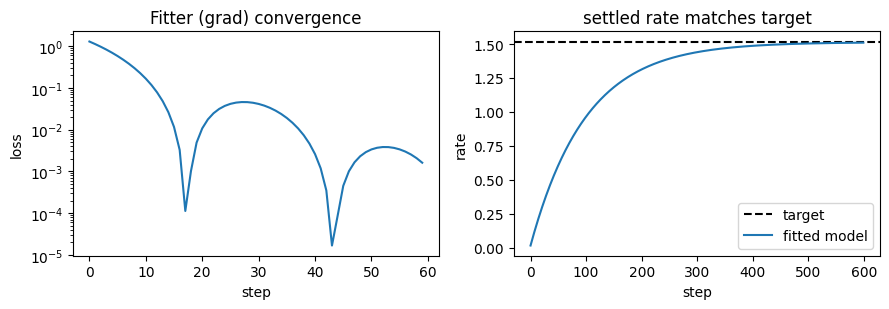
FitResult(backend='grad', best_loss=1.66887e-05, n_steps=60, params=[g])
recovered g = {'g': 1.9878}
best loss   = 1.6688674804754555e-05

fig, ax = plt.subplots(1, 2, figsize=(9, 3.2))
ax[0].plot(result.history)
ax[0].set(xlabel='step', ylabel='loss', title='Fitter (grad) convergence')
ax[0].set_yscale('log')
ax[1].axhline(float(target_amp), ls='--', c='k', label='target')
ax[1].plot(u.get_magnitude(predict(model)), label='fitted model')
ax[1].set(xlabel='step', ylabel='rate', title='settled rate matches target')
ax[1].legend()
fig.tight_layout()

3b. The same fit, hand-written

Fitter’s 'grad' backend is this loop. Writing it out is worth doing once, because the moment you need something Fitter does not expose – minibatches, an epoch loop, a held-out metric – you drop down to exactly this and add your own control flow. The five lines that matter:

1. weights = model.states(brainstate.ParamState) – the trainable leaves.

2. optimizer.register_trainable_weights(weights).

3. a loss closure run inside model.param_precompute() (applies transforms / precompute), adding model.reg_loss().

4. brainstate.transform.grad(loss, weights, return_value=True).

5. optimizer.step(grads) – all wrapped in brainstate.transform.jit.

model2 = GainPopulation(1, g=0.5)
weights = model2.states(brainstate.ParamState)
optimizer = braintools.optim.Adam(lr=0.1)
optimizer.register_trainable_weights(weights)

def loss_closure():
    with model2.param_precompute():
        loss = steadystate_loss()(predict(model2), target_amp)
        return loss + model2.reg_loss()

@brainstate.transform.jit
def train_step():
    grad_fn = brainstate.transform.grad(loss_closure, weights, return_value=True)
    grads, loss = grad_fn()
    optimizer.step(grads)
    return loss

history = [float(train_step()) for _ in range(60)]
print('hand-rolled g =', round(float(model2.g.value()), 4))
print('final loss    =', history[-1])
# Same key gotcha: a standalone grad is keyed by the ParamState tuple, not 'g'.
grad_fn = brainstate.transform.grad(loss_closure, weights, return_value=True)
grads, _ = grad_fn()
print('raw grad keys =', list(grads.keys()))

hand-rolled g = 1.9546
final loss    = 0.0016139140352606773

raw grad keys = [('g', 'val')]

Both paths converge to the same g ~ 2.0. The hand-rolled loop is the template a task-shaped trainer extends – see the final section, Where this is going.

4. Batch the search with vmap

To evaluate the loss across many parameter values at once, vmap over parameters – build a fresh model inside the mapped function and map over the scalar. This is the supported batching axis. (Batching states through init_all_states(batch_size=...) is the right tool for an ensemble of one model, but a delay-coupled network’s prefetch does not vectorise that way – vmap over parameters instead.)

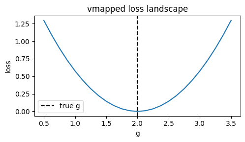
def loss_at(g_value):
    m = GainPopulation(1, g=g_value)
    return steadystate_loss()(predict(m), target_amp)

grid = jnp.linspace(0.5, 3.5, 25)
losses = jax.vmap(loss_at)(grid)        # all 25 evaluated in one compiled call
best = grid[jnp.argmin(losses)]
print('vmap grid minimum at g =', round(float(best), 3))

plt.figure(figsize=(5, 3))
plt.plot(grid, losses)
plt.axvline(2.0, ls='--', c='k', label='true g')
plt.xlabel('g'); plt.ylabel('loss'); plt.title('vmapped loss landscape')
plt.legend(); plt.tight_layout()

vmap grid minimum at g = 2.0

Where this is going

Everything above is the stable, public contract:

Piece	API
trainable parameter	Param(value, fit=True)
loss	objectives-style callable(prediction, target)
one-call fit	brainmass.Fitter(...).fit(target=...)
custom loop	states(ParamState) -> register_trainable_weights -> grad -> step
batched search	jax.vmap over parameters

Fitter fits one fixed target – a single predict(model) -> prediction compared against one target. Task training (minibatched (inputs, targets), an epoch loop, a held-out metric) is not something Fitter exposes; you reach for the hand-written loop in section 3b and add the batching yourself.

That gap is named and given a home – but deliberately not built yet – as the deferred Trainer in the Data-Driven Modeling Roadmap. A future goal will build the Trainer (and model-discovery tooling) against this exact contract: it wraps the section-3b loop plus batched state initialisation, and registers its datasets through brainmass.datasets. Authoring a custom model, objective, and loop the way this guide does is precisely what makes it slot in without restructuring.

See Also

• Creating Custom Models – the model contract this builds on.

• Creating an Objective – the objective contract in depth.

• Data-Driven Modeling – the data-driven pillar and its roadmap.

• Fitting with Gradients – a worked end-to-end fit.