Harmonic Oscillator Recurrent Network (HORN)

HORN is a recurrent network of damped, driven harmonic oscillators used as a trainable dynamical reservoir / sequence model. Each unit is a second-order oscillator with position \(x\) and velocity \(y\),

\[\ddot x + \gamma\,\dot x + \omega^2 x = \alpha\,\phi(\text{input} + \text{recurrent}),\]

so the network embeds inputs into a bank of coupled resonators. Stacked as HORNSeqLayer / HORNSeqNetwork, it can be trained on sequence tasks (see the Training on tasks tutorial). Here we drive a single HORNStep layer and watch its oscillatory hidden state.

Reference: Effenberger, Carvalho, Jain et al. (2025), A biology-inspired recurrent oscillator network for computations in high-dimensional state space (HORN), bioRxiv.

Build the model

A single HORN layer with in_size = 16 oscillatory units. We raise alpha to make the response visibly oscillatory.

node = brainmass.HORNStep(in_size=16, alpha=0.3)
node

HORNStep(
  in_size=(16,),
  out_size=(16,),
  alpha=Const(
    fit=False,
    t=IdentityT(),
    reg=None,
    val=Array(0.3, dtype=float32)
  ),
  omega=Const(
    fit=False,
    t=IdentityT(),
    reg=None,
    val=Array(0.22439948, dtype=float32)
  ),
  gamma=Const(
    fit=False,
    t=IdentityT(),
    reg=None,
    val=Array(0.01, dtype=float32)
  ),
  v=Const(
    fit=False,
    t=IdentityT(),
    reg=None,
    val=Array(0., dtype=float32)
  ),
  x_init=Constant(value=0.0),
  y_init=Constant(value=0.0)
)

Run a simulation

We drive the layer with a brief input pulse and let it ring down — a sequence model’s impulse response. HORNStep.update(inputs) takes one positional input, so we provide it via the Simulator’s inputs callable.

def pulse(i, t):
    on = (t >= 5. * u.ms) & (t < 8. * u.ms)
    return jnp.where(on, 1.0, 0.0) * jnp.ones((16,))

sim = brainmass.Simulator(node, dt=0.1 * u.ms)
res = sim.run(120. * u.ms, inputs=pulse, monitors=['x', 'y'])
res['x'].shape

(1200, 16)

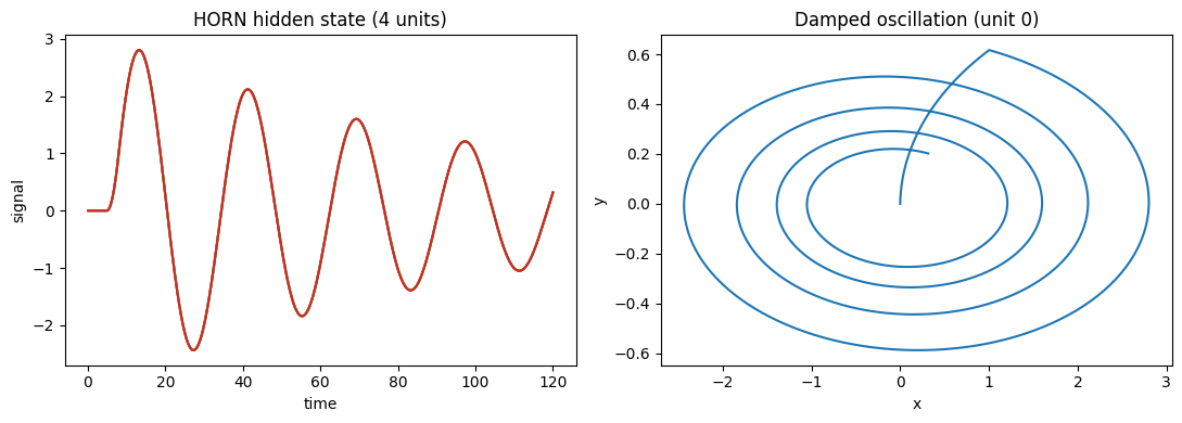
Visualize

Left: the position state of a few units ringing after the pulse. Right: a position-velocity phase portrait of one unit spiraling toward rest.

fig, axes = plt.subplots(1, 2, figsize=(11, 4))
brainmass.viz.plot_timeseries(res['x'][:, :4], ts=res['ts'], ax=axes[0])
axes[0].set_title('HORN hidden state (4 units)')
brainmass.viz.plot_phase_portrait(res['x'][:, 0], res['y'][:, 0], ax=axes[1])
axes[1].set_xlabel('x'); axes[1].set_ylabel('y')
axes[1].set_title('Damped oscillation (unit 0)')
plt.tight_layout()
plt.show()

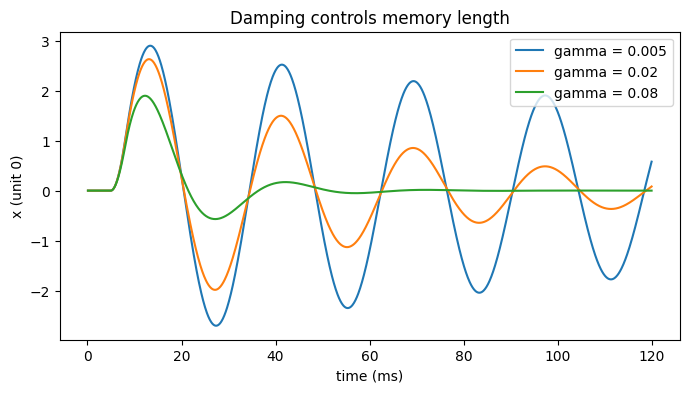
Try it: vary the damping gamma

More damping makes the impulse response decay faster (shorter memory); less damping lets the oscillators ring longer. The sequence-model variants HORNSeqLayer and HORNSeqNetwork stack these units and add trainable input/recurrent/output weights — see Training on Tasks.

fig, ax = plt.subplots(figsize=(8, 4))
for gamma in [0.005, 0.02, 0.08]:
    m = brainmass.HORNStep(in_size=16, alpha=0.3, gamma=gamma)
    r = brainmass.Simulator(m, dt=0.1 * u.ms).run(120. * u.ms, inputs=pulse,
                                                  monitors=['x'])
    ax.plot(u.get_magnitude(r['ts']), u.get_magnitude(r['x'])[:, 0],
            label=f'gamma = {gamma}')
ax.set_xlabel('time (ms)'); ax.set_ylabel('x (unit 0)'); ax.legend()
ax.set_title('Damping controls memory length')
plt.show()