Your First Simulation

Welcome to brainmass. In this first tutorial you will run a single neural-mass model from start to finish using only the high-level API — no hand-written integration loops. By the end you will be able to:

1. construct a model and initialise its state,

2. run it for a chosen duration with the Simulator,

3. plot the result with brainmass.viz, and

4. change one parameter and re-run to see the effect.

We will use the FitzHughNagumoStep model — a classic two-variable model of an excitable unit. It sits quietly at rest until a stimulus pushes it past a threshold, at which point it fires a single large excursion (a “spike”) before relaxing back. That makes the effect of a parameter change easy to see.

Note

Every code cell on this page is executed when the notebook is authored, so the outputs you see are real. For the 10-minute tour of the whole library — networks, noise, and gradient-based fitting — see Quickstart.

Setup

We import brainmass and a few companions. brainunit (u) gives us unit-aware quantities: the time step dt and the run duration are physical times like 0.1 * u.ms, not bare numbers. We set a global dt once through the environment; the Simulator also takes it explicitly below.

import brainmass
import brainstate
import brainunit as u
import jax.numpy as jnp
import matplotlib.pyplot as plt

brainstate.environ.set(dt=0.1 * u.ms)
brainmass.__version__

An NVIDIA GPU may be present on this machine, but a CUDA-enabled jaxlib is not installed. Falling back to cpu.

'0.0.6'

1. Construct a model

A brainmass model is a *Step object — one update step of a neural-mass equation, sized for in_size regions. Here we build a single FitzHugh–Nagumo unit (in_size=1). It carries two state variables: a fast activator V (membrane-potential–like) and a slow recovery variable w.

node = brainmass.FitzHughNagumoStep(in_size=1)
node

FitzHughNagumoStep(
  in_size=(1,),
  out_size=(1,),
  alpha=Const(
    fit=False,
    t=IdentityT(),
    reg=None,
    val=Array(3., dtype=float32)
  ),
  beta=Const(
    fit=False,
    t=IdentityT(),
    reg=None,
    val=Array(4., dtype=float32)
  ),
  gamma=Const(
    fit=False,
    t=IdentityT(),
    reg=None,
    val=Array(-1.5, dtype=float32)
  ),
  delta=Const(
    fit=False,
    t=IdentityT(),
    reg=None,
    val=Array(0., dtype=float32)
  ),
  epsilon=Const(
    fit=False,
    t=IdentityT(),
    reg=None,
    val=Array(0.5, dtype=float32)
  ),
  tau=Const(
    fit=False,
    t=IdentityT(),
    reg=None,
    val=Quantity(20., "ms")
  ),
  init_V=Uniform(low=0, high=0.05),
  init_w=Uniform(low=0, high=0.05),
  method=exp_euler
)

2. Run it with the Simulator

The Simulator owns the whole run loop. A single .run(...) call:

• sets dt and initialises the model’s state (init_all_states),

• steps the model forward, and

• returns the recorded trajectories as a plain dict.

How many steps is that? The number of integration steps is duration / dt. With duration = 200 * u.ms and dt = 0.1 * u.ms that is 2000 steps.

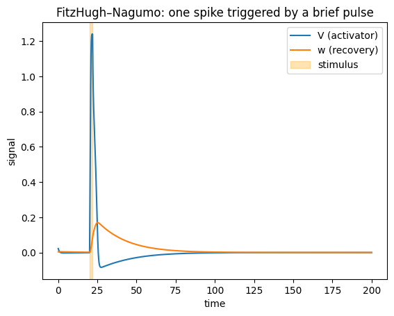
We give the unit a brief external stimulus: a current pulse to V between 20 ms and 22 ms, via the inputs= callback (it receives the step index i and time t and returns the drive for that step). We record both state variables by name with monitors=['V', 'w'].

def stimulus(i, t):
    """A brief supra-threshold current pulse to V between 20 and 22 ms."""
    pulse = jnp.where((t > 20.0 * u.ms) & (t < 22.0 * u.ms), 1.5, 0.0)
    return (pulse,)

sim = brainmass.Simulator(node, dt=0.1 * u.ms)
res = sim.run(200.0 * u.ms, inputs=stimulus, monitors=["V", "w"])

print("recorded keys:", list(res))
print("V trajectory shape (steps, regions):", res["V"].shape)
print("time axis runs from", res["ts"][0], "to", res["ts"][-1])

recorded keys: ['V', 'w', 'ts']
V trajectory shape (steps, regions): (2000, 1)
time axis runs from 0.1 ms to 200. ms

3. Plot the result

brainmass.viz.plot_timeseries() takes the trajectory and the time axis directly. The single sub-threshold rest is interrupted by one clean spike right after the 20 ms pulse — the hallmark of an excitable unit.

ax = brainmass.viz.plot_timeseries(
    res["V"], ts=res["ts"], labels=["V (activator)"]
)
brainmass.viz.plot_timeseries(res["w"], ts=res["ts"], labels=["w (recovery)"], ax=ax)
ax.axvspan(20, 22, color="orange", alpha=0.3, label="stimulus")
ax.legend()
ax.set_title("FitzHugh–Nagumo: one spike triggered by a brief pulse");

A note on transients

Models often start away from their natural operating point and need a few milliseconds to settle. That initial transient is usually not interesting, so the Simulator can discard it for you: pass transient=<duration> and the first stretch is dropped from the returned arrays (the run itself is unchanged — only the output is trimmed).

res_full = sim.run(200.0 * u.ms, inputs=stimulus, monitors=["V"])
res_trim = sim.run(200.0 * u.ms, inputs=stimulus, monitors=["V"], transient=50.0 * u.ms)

print("without transient discard:", res_full["V"].shape[0], "recorded steps")
print("with 50 ms discarded:    ", res_trim["V"].shape[0], "recorded steps")
print("first recorded time now starts at", res_trim["ts"][0])

without transient discard: 2000 recorded steps
with 50 ms discarded:     1500 recorded steps
first recorded time now starts at 50.1 ms

4. Change one parameter and see the effect

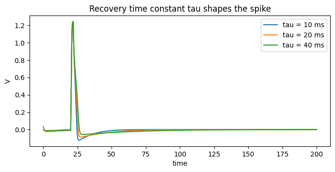
The point of a model is that its parameters control its behaviour. The recovery time constant tau sets how quickly the slow variable w chases the activator. Make tau larger and recovery is sluggish, so the spike is broader; make it smaller and the unit snaps back faster.

We build the same model three times with different tau, run each, and overlay the activator traces. Constructing-running-plotting is so concise that a parameter sweep is just a loop over model builds.

fig, ax = plt.subplots(figsize=(8, 3.5))

for tau in [10.0, 20.0, 40.0]:
    model = brainmass.FitzHughNagumoStep(in_size=1, tau=tau * u.ms)
    r = brainmass.Simulator(model, dt=0.1 * u.ms).run(
        200.0 * u.ms, inputs=stimulus, monitors=["V"]
    )
    brainmass.viz.plot_timeseries(
        r["V"], ts=r["ts"], labels=[f"tau = {tau:.0f} ms"], ax=ax
    )

ax.set_title("Recovery time constant tau shapes the spike")
ax.set_ylabel("V");

What you learned

• A model is a *Step object sized for in_size regions.

• Simulator(model, dt=...).run(duration, monitors=...) initialises, steps, and collects trajectories — duration / dt gives the number of steps.

• monitors=[...] records named state variables; inputs= injects an external drive; transient= trims the warm-up from the output.

• brainmass.viz turns trajectories into plots in one line.

• Changing a parameter and re-running is the basic loop of model exploration.

Next steps

• Models and Dynamics — tour the model families and watch a parameter move a system across a bifurcation.

• Noise and Stochastic Runs — add stochastic fluctuations.

• Gallery — a runnable demo for every model in the library.