From Activity to Signals

Neural mass models produce neural activity — firing rates, membrane potentials, synaptic currents. But experiments do not measure activity directly; they measure signals: a BOLD time course from fMRI, voltages from EEG, magnetic fields from MEG. A forward model is the biophysics that turns simulated activity into a predicted signal, so a model can be compared to (and fit against) real data.

This page explains the theory of the two forward models brainmass ships — the hemodynamic (BOLD) model and the electromagnetic (EEG/MEG) lead-field model — what each observable measures, and the assumptions baked into each. The hands-on version is Forward Models; the architectural role of this layer is in Architecture Overview.

The forward-model idea

Every forward model is a map

\[ \text{neural activity } a(t) \;\xrightarrow{\;\text{biophysics}\;}\; \text{signal } y(t). \]

What distinguishes the modalities is what physics does the mapping and what is actually measured:

Modality	Measures	Forward physics	Timescale
fMRI / BOLD	blood-oxygenation changes	neurovascular coupling (hemodynamics)	seconds (slow)
EEG	scalp electric potential	volume conduction of dipolar currents	milliseconds (fast)
MEG	extracranial magnetic field	magnetic field of the same currents	milliseconds (fast)

In brainmass every forward model is itself a differentiable module, so a loss defined in signal space (BOLD, EEG, or MEG) backpropagates all the way to the underlying neural parameters — the end-to-end differentiability discussed in Why Differentiable?.

BOLD: the hemodynamic forward model

fMRI does not see neurons; it sees blood. Local neural activity raises metabolic demand, which (via neurovascular coupling) increases blood flow, blood volume, and the local ratio of oxygenated to deoxygenated haemoglobin. Because oxygenated and deoxygenated blood have different magnetic susceptibilities, this changes the MR signal — the blood-oxygen-level-dependent (BOLD) contrast. The forward model is the chain activity → flow → volume & deoxyhaemoglobin → BOLD.

The Balloon–Windkessel model

brainmass.BOLDSignal implements the Balloon–Windkessel model of Friston et al. (2003). For each region, synaptic activity \(z_i\) drives a vasodilatory signal \(x_i\), which changes inflow \(f_i\), blood volume \(v_i\), and deoxyhaemoglobin content \(q_i\):

\[\begin{split} \begin{aligned} \dot{x}_i &= z_i - \kappa_i x_i - \gamma_i (f_i - 1), \\ \dot{f}_i &= x_i, \\ \tau_i \dot{v}_i &= f_i - v_i^{1/\alpha}, \\ \tau_i \dot{q}_i &= \frac{f_i}{\rho}\bigl[1 - (1-\rho)^{1/f_i}\bigr] - q_i\,v_i^{\,1/\alpha - 1}, \end{aligned} \end{split}\]

with the measured BOLD a static nonlinear read-out of volume and deoxyhaemoglobin,

\[ \mathrm{BOLD}_i = V_0\bigl[k_1(1 - q_i) + k_2(1 - q_i/v_i) + k_3(1 - v_i)\bigr], \]

where \(\rho\) is the resting oxygen-extraction fraction, \(\alpha\) is Grubb’s exponent, \(\tau\) the hemodynamic transit time, and \(k_1, k_2, k_3\) are fixed biophysical constants. The key assumptions: the response is regional and local (no hemodynamic coupling between regions), and it is a slow temporal low-pass — the haemodynamics blur fast neural dynamics into a response that peaks several seconds after activity.

The convolution (HRF) shortcut

The full ODE is detailed but stiff and slow. For fitting, brainmass also offers HRFBold: a single linear convolution of (downsampled) activity with a closed-form hemodynamic response function \(h(t)\),

\[ \mathrm{BOLD}(t) = k_1 V_0\,\bigl(h * y_{\downarrow}\bigr)(t) - 1, \]

using kernels such as the canonical first-order Volterra (damped oscillator) or a mixture of gammas. This is fast, simple, and differentiable in its handful of scalar parameters — the right tool when the BOLD model sits inside an optimisation loop. Empirically the two routes track each other closely (best-lag correlation \(\approx 0.98\) on a slow drive), differing mainly in their intrinsic latency. So: BOLDSignal when biophysical realism matters, HRFBold when you are fitting.

import brainmass
import brainunit as u
import numpy as np
import matplotlib.pyplot as plt

# Visualise a canonical hemodynamic response function: the impulse response that
# convolution-BOLD applies to neural activity. Note the ~5-6 s peak and post-undershoot.
kernel = brainmass.MixtureOfGammasHRFKernel()
t = np.linspace(0.0, 25.0, 400) * u.second
h = kernel(t)

fig, ax = plt.subplots(figsize=(7, 4))
ax.plot(np.asarray(t.to_decimal(u.second)), np.asarray(h))
ax.axhline(0.0, color='0.7', lw=0.8)
ax.set_xlabel('time after a brief neural event (s)')
ax.set_ylabel('hemodynamic response $h(t)$')
ax.set_title('Canonical HRF: activity is blurred & delayed by ~5 s')
fig.tight_layout()
plt.show()

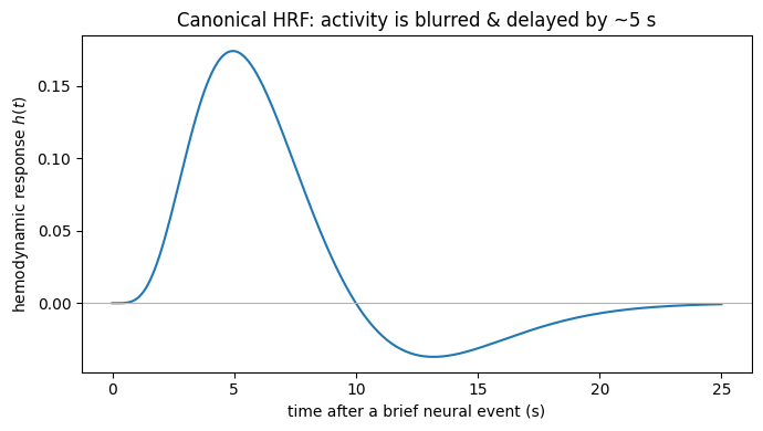
The HRF makes the BOLD assumptions visceral: a brief burst of neural activity produces a response that peaks several seconds later and undershoots before returning to baseline. fMRI therefore reports a slow, lagged, smoothed image of the underlying fast dynamics — which is exactly why whole-brain BOLD models compare functional connectivity (correlation structure over minutes) rather than millisecond waveforms.

EEG / MEG: the lead-field forward model

EEG and MEG see electromagnetism. Synchronous post-synaptic currents in populations of pyramidal neurons act, at a distance, like equivalent current dipoles (ECDs). Each region’s dipole sets up an electric potential (measured by EEG electrodes) and a magnetic field (measured by MEG sensors) throughout the head. Because the quasi-static Maxwell equations are linear, the mapping from source currents to sensors is a single matrix multiply.

The lead-field equation

brainmass’s LeadFieldModel implements

\[ \mathbf{y}(t) \;=\; \mathbf{s}(t)\,\mathbf{L} \;+\; \boldsymbol{\varepsilon}(t), \]

where

• \(\mathbf{s}(t) \in \mathbb{R}^{R}\) is the equivalent current dipole moment per region (typically in \(\mathrm{nA\cdot m}\)), obtained from the NMM observable via a scale factor.

• \(\mathbf{L} \in \mathbb{R}^{R \times M}\) is the lead-field (gain) matrix — the signal each unit dipole produces at each of \(M\) sensors. Its units are \(\mathrm{V/(nA\cdot m)}\) for EEG and \(\mathrm{T/(nA\cdot m)}\) for MEG.

• \(\mathbf{y}(t) \in \mathbb{R}^{M}\) are the sensor measurements (volts for EEG, tesla for MEG).

• \(\boldsymbol{\varepsilon}(t) \sim \mathcal{N}(\mathbf{0}, \boldsymbol{\Sigma})\) is additive sensor noise.

The lead field \(\mathbf{L}\) encodes all the head geometry and physics — the conductivity of brain, skull, and scalp; sensor positions; source orientations — and is normally precomputed by a head model (boundary- or finite-element method) in a tool such as MNE, FieldTrip, or Brainstorm. brainmass consumes that \(\mathbf{L}\) and provides the differentiable, unit-safe projection, aggregating vertex-level lead fields to region level when needed.

What each modality assumes — and how they differ

The same dipolar sources feed both EEG and MEG, but the physics treats them differently:

• EEG measures scalp potential. The currents must cross the skull, whose low conductivity smears the potential — EEG has lower spatial resolution but sees all source orientations, including radial (pointing out of the head).

• MEG measures the magnetic field, which the skull barely perturbs (magnetic permeability is nearly uniform), so MEG is less smeared. But a radially-oriented dipole in a spherically symmetric head produces no external magnetic field — MEG is largely blind to radial sources and most sensitive to tangential ones.

Shared assumptions: the quasi-static approximation (no wave propagation at these frequencies, so the map is an instantaneous linear projection), a fixed source space (one dipole per region, with a chosen orientation), and a head conductivity model. These assumptions are what make the forward map a constant matrix \(\mathbf{L}\) — and what make the inverse problem (recovering sources from sensors) ill-posed, which is precisely why a generative forward model like this one is useful.

A units caveat worth flagging (see Forward Models): the EEGLeadFieldModel helper is tuned for an mV neural source. For MEG from an mV source, drive the base LeadFieldModel with an explicit scale and sensor_unit=u.tesla so the output lands in tesla.

import brainmass
import brainstate
import brainunit as u
import numpy as np
import jax.numpy as jnp

brainstate.random.seed(0)

# A tiny EEG forward projection: R=4 source regions -> M=6 sensors.
# The lead field carries the EEG sensor unit per dipole moment, mV / (nA*m).
R, M = 4, 6
L = jnp.asarray(np.random.randn(R, M)) * (u.mV / (u.nA * u.meter))
eeg = brainmass.EEGLeadFieldModel(in_size=(R,), out_size=(M,), L=L)

# A short window of regional dipole activity (mV NMM observable), (T, R).
T = 50
sources = (jnp.array([1.0, -0.5, 0.8, 0.2]) * jnp.ones((T, R))) * u.mV
sensors = eeg.update(sources)   # linear lead-field projection -> sensor space

print('source activity (T x R):', sources.shape, ' ->  sensors (T x M):', sensors.shape)
print('sensor output unit:', u.get_unit(sensors))   # mV, via s @ L

source activity (T x R): (50, 4)  ->  sensors (T x M): (50, 6)
sensor output unit: mV

The four regional sources are linearly mixed by the lead field into six sensor measurements, unit-correctly (volts out). The same \(\mathbf{L}\)-style multiply, with a tesla-valued lead field, gives MEG. Because the projection is differentiable, a loss on the sensor signal flows back to the neural model — closing the loop from parameters all the way to the measured signal.

Choosing a forward model

You are modelling…	Use	Why
Resting-state fMRI / BOLD FC	BOLDSignal or HRFBold	hemodynamics; FC over minutes
Fitting in BOLD space	HRFBold	fast, differentiable convolution
Biophysically realistic BOLD	BOLDSignal	full Balloon–Windkessel ODE
EEG (scalp potentials)	EEGLeadFieldModel	volume conduction, all orientations
MEG (magnetic fields)	LeadFieldModel / MEGLeadFieldModel	tangential-source sensitivity

In all cases the forward model is the generative link between a neural mass model and data — and in brainmass it is one more differentiable module in the chain, not a separate post-processing step.

Key takeaways

• A forward model maps simulated neural activity to a measured signal; the modality determines the physics and what is observed.

• BOLD is hemodynamic, regional, and slow: a Balloon–Windkessel ODE (BOLDSignal) or an HRF convolution (HRFBold) that blurs and delays activity by seconds.

• EEG/MEG are electromagnetic and fast: a linear lead-field projection of dipolar source currents, with EEG smeared by the skull and MEG blind to radial sources.

• Every forward model in brainmass is differentiable and unit-safe, so signal-space losses backpropagate to neural parameters.

See also

• Forward Models — running BOLD and EEG/MEG forward models.

• Architecture Overview — the observation layer’s place in the stack.

• Why Differentiable? — why end-to-end differentiability matters.

• API Reference — the forward-model and observation API.

References

• Friston, K. J., Harrison, L., & Penny, W. (2003). Dynamic causal modelling. NeuroImage, 19(4), 1273–1302.

• Buxton, R. B., Wong, E. C., & Frank, L. R. (1998). Dynamics of blood flow and oxygenation changes during brain activation: the balloon model. Magnetic Resonance in Medicine, 39(6), 855–864.

• Hämäläinen, M., Hari, R., Ilmoniemi, R. J., Knuutila, J., & Lounasmaa, O. V. (1993). Magnetoencephalography — theory, instrumentation, and applications to noninvasive studies of the working human brain. Reviews of Modern Physics, 65(2), 413–497.

• Nunez, P. L., & Srinivasan, R. (2006). Electric Fields of the Brain: The Neurophysics of EEG (2nd ed.). Oxford University Press.