Larter-Breakspear Model

The Larter-Breakspear model is a conductance-based mean-field model derived from the Morris-Lecar equations, with mean membrane potential \(V\), a potassium gating variable \(W\), and an inhibitory variable \(Z\). Voltage-gated Na\(^+\), K\(^+\) and Ca\(^{2+}\) currents make it capable of fixed points, limit cycles, and chaos depending on parameters. The pyramidal firing-threshold variance \(d_V\) is a particularly effective knob for selecting the dynamical regime.

Reference: Breakspear, Terry & Friston (2003), Modulation of excitatory synaptic coupling facilitates synchronization and complex dynamics in a biophysical model of neuronal dynamics, Network: Computation in Neural Systems 14(4):703-732.

Build the model

We pick d_V = 0.57, which puts the node in a limit-cycle band.

node = brainmass.LarterBreakspearStep(in_size=1, d_V=0.57)
node

LarterBreakspearStep(
  in_size=(1,),
  out_size=(1,),
  gCa=Const(
    fit=False,
    t=IdentityT(),
    reg=None,
    val=Array(1.1, dtype=float32)
  ),
  gK=Const(
    fit=False,
    t=IdentityT(),
    reg=None,
    val=Array(2., dtype=float32)
  ),
  gL=Const(
    fit=False,
    t=IdentityT(),
    reg=None,
    val=Array(0.5, dtype=float32)
  ),
  gNa=Const(
    fit=False,
    t=IdentityT(),
    reg=None,
    val=Array(6.7, dtype=float32)
  ),
  TCa=Const(
    fit=False,
    t=IdentityT(),
    reg=None,
    val=Array(-0.01, dtype=float32)
  ),
  TK=Const(
    fit=False,
    t=IdentityT(),
    reg=None,
    val=Array(0., dtype=float32)
  ),
  TNa=Const(
    fit=False,
    t=IdentityT(),
    reg=None,
    val=Array(0.3, dtype=float32)
  ),
  d_Ca=Const(
    fit=False,
    t=IdentityT(),
    reg=None,
    val=Array(0.15, dtype=float32)
  ),
  d_K=Const(
    fit=False,
    t=IdentityT(),
    reg=None,
    val=Array(0.3, dtype=float32)
  ),
  d_Na=Const(
    fit=False,
    t=IdentityT(),
    reg=None,
    val=Array(0.15, dtype=float32)
  ),
  VCa=Const(
    fit=False,
    t=IdentityT(),
    reg=None,
    val=Array(1., dtype=float32)
  ),
  VK=Const(
    fit=False,
    t=IdentityT(),
    reg=None,
    val=Array(-0.7, dtype=float32)
  ),
  VL=Const(
    fit=False,
    t=IdentityT(),
    reg=None,
    val=Array(-0.5, dtype=float32)
  ),
  VNa=Const(
    fit=False,
    t=IdentityT(),
    reg=None,
    val=Array(0.53, dtype=float32)
  ),
  phi=Const(
    fit=False,
    t=IdentityT(),
    reg=None,
    val=Array(0.7, dtype=float32)
  ),
  tau_K=Const(
    fit=False,
    t=IdentityT(),
    reg=None,
    val=Array(1., dtype=float32)
  ),
  aee=Const(
    fit=False,
    t=IdentityT(),
    reg=None,
    val=Array(0.4, dtype=float32)
  ),
  aei=Const(
    fit=False,
    t=IdentityT(),
    reg=None,
    val=Array(2., dtype=float32)
  ),
  aie=Const(
    fit=False,
    t=IdentityT(),
    reg=None,
    val=Array(2., dtype=float32)
  ),
  ane=Const(
    fit=False,
    t=IdentityT(),
    reg=None,
    val=Array(1., dtype=float32)
  ),
  ani=Const(
    fit=False,
    t=IdentityT(),
    reg=None,
    val=Array(0.4, dtype=float32)
  ),
  b=Const(
    fit=False,
    t=IdentityT(),
    reg=None,
    val=Array(0.1, dtype=float32)
  ),
  C=Const(
    fit=False,
    t=IdentityT(),
    reg=None,
    val=Array(0.1, dtype=float32)
  ),
  Iext=Const(
    fit=False,
    t=IdentityT(),
    reg=None,
    val=Array(0.3, dtype=float32)
  ),
  rNMDA=Const(
    fit=False,
    t=IdentityT(),
    reg=None,
    val=Array(0.25, dtype=float32)
  ),
  VT=Const(
    fit=False,
    t=IdentityT(),
    reg=None,
    val=Array(0., dtype=float32)
  ),
  d_V=Const(
    fit=False,
    t=IdentityT(),
    reg=None,
    val=Array(0.57, dtype=float32)
  ),
  ZT=Const(
    fit=False,
    t=IdentityT(),
    reg=None,
    val=Array(0., dtype=float32)
  ),
  d_Z=Const(
    fit=False,
    t=IdentityT(),
    reg=None,
    val=Array(0.7, dtype=float32)
  ),
  QV_max=Const(
    fit=False,
    t=IdentityT(),
    reg=None,
    val=Array(1., dtype=float32)
  ),
  QZ_max=Const(
    fit=False,
    t=IdentityT(),
    reg=None,
    val=Array(1., dtype=float32)
  ),
  t_scale=Const(
    fit=False,
    t=IdentityT(),
    reg=None,
    val=Array(1., dtype=float32)
  ),
  init_V=Constant(value=0.0),
  init_W=Constant(value=0.0),
  init_Z=Constant(value=0.0),
  method=exp_euler
)

Run a simulation

sim = brainmass.Simulator(node, dt=0.1 * u.ms)
res = sim.run(500. * u.ms, monitors=['V', 'W'], transient=100. * u.ms)
res['V'].shape

(4000, 1)

Visualize

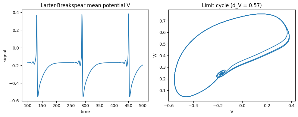
The mean potential V oscillates; the V-W phase portrait shows the conductance-based limit cycle.

fig, axes = plt.subplots(1, 2, figsize=(10, 4))
brainmass.viz.plot_timeseries(res['V'], ts=res['ts'], ax=axes[0])
axes[0].set_title('Larter-Breakspear mean potential V')
brainmass.viz.plot_phase_portrait(res['V'], res['W'], ax=axes[1])
axes[1].set_xlabel('V'); axes[1].set_ylabel('W')
axes[1].set_title('Limit cycle (d_V = 0.57)')
plt.tight_layout()
plt.show()

Try it: vary the threshold variance d_V

The regime boundaries are sharp. d_V = 0.65 (default) gives a fixed point; d_V = 0.57 gives a limit cycle. We report the steady-state standard deviation of V as a simple oscillation detector.

for d_V in [0.50, 0.57, 0.65]:
    m = brainmass.LarterBreakspearStep(in_size=1, d_V=d_V)
    r = brainmass.Simulator(m, dt=0.1 * u.ms).run(
        500. * u.ms, monitors=['V'], transient=200. * u.ms)
    std = float(np.std(u.get_magnitude(r['V'])))
    regime = 'oscillatory' if std > 1e-3 else 'fixed point'
    print(f'd_V = {d_V:.2f}  ->  std(V) = {std:.3e}  ({regime})')

d_V = 0.50  ->  std(V) = 2.363e-06  (fixed point)
d_V = 0.57  ->  std(V) = 1.110e-01  (oscillatory)

d_V = 0.65  ->  std(V) = 1.307e-01  (oscillatory)