Why Differentiable?

This is the page that explains what makes brainmass different. Other whole-brain toolkits run forward simulations and fit parameters with grid or evolutionary search. brainmass is built on JAX, so its entire pipeline — parameters → ODE solve → coupling → forward model → signal — is differentiable. You can backpropagate through the ODE solve and obtain the exact gradient of a loss with respect to every parameter at once.

That single capability changes how you fit, scale, and even train neural mass models. This page builds the intuition, walks through the new application scenarios it unlocks, and places brainmass next to The Virtual Brain and neurolib with a conservative comparison.

The core idea: backprop through the solve

A whole-brain simulation is a long composition of differentiable operations. A fixed-step solver advances the state \(s\) by repeatedly applying an update map,

\[ s_{t+1} = \Phi(s_t, \theta), \qquad t = 0, 1, \dots, T-1, \]

where \(\theta\) collects all parameters (local model parameters, coupling strength, forward-model constants). A scalar loss \(\mathcal{L}\) compares the resulting signal to data. Because every step \(\Phi\) is differentiable, the whole rollout is differentiable, and the chain rule gives

\[ \frac{\partial \mathcal{L}}{\partial \theta} = \sum_{t} \frac{\partial \mathcal{L}}{\partial s_T} \left(\prod_{k>t} \frac{\partial \Phi}{\partial s_k}\right) \frac{\partial \Phi}{\partial \theta}. \]

Reverse-mode automatic differentiation (backpropagation through time) computes this entire sum in one backward pass whose cost is a small constant multiple of the forward simulation — independent of the number of parameters. JAX builds the backward pass automatically; you never write it.

Contrast this with the standard alternatives:

• Grid search evaluates the loss on a lattice of parameter values. The number of points grows as \((\text{resolution})^{\,d}\) in the parameter dimension \(d\) — the curse of dimensionality. Feasible for 1–2 parameters, hopeless for many.

• Evolutionary / derivative-free search (CMA-ES, differential evolution, Nevergrad) needs many forward evaluations to estimate a good direction, and the count climbs steeply with \(d\). Robust and gradient-free, but sample-hungry.

A gradient points directly downhill. Instead of probing the loss landscape with hundreds of blind forward runs, you get the steepest-descent direction from a single forward+backward pass and step along it.

A picture: gradient vs blind search

Consider fitting a single parameter (a region’s Hopf bifurcation parameter \(a\)) so that the model’s settled oscillation amplitude matches a target. The loss is a smooth bowl in \(a\). A gradient tells us the slope at our current guess for free (one backward pass); grid/evolutionary methods would instead sample the bowl at many points to infer the same direction. Let’s visualise that loss surface and the exact gradient at one point.

import brainmass
import brainstate
import braintools
import brainunit as u
import jax
import jax.numpy as jnp

brainstate.random.seed(0)
brainstate.environ.set(dt=0.1 * u.ms)


def settled_amplitude(a_value):
    # Build the model INSIDE the loss so the swept scalar is differentiated.
    node = brainmass.HopfStep(in_size=1, a=a_value, w=0.3,
                              init_x=braintools.init.Constant(0.5))
    res = brainmass.Simulator(node, dt=0.1 * u.ms).run(
        400 * u.ms, monitors=['x'], transient=200 * u.ms)
    x = u.get_magnitude(res['x'])           # strip units before the reduction
    return jnp.sqrt(jnp.mean(x ** 2)) * jnp.sqrt(2.0)   # RMS -> amplitude


target = 1.0  # amplitude we want to match

def loss(a_value):
    return (settled_amplitude(a_value) - target) ** 2

# The exact gradient of the loss wrt `a`, by backprop THROUGH the 2000-step solve.
a0 = 0.4
g = jax.grad(loss)(a0)
print(f'loss({a0}) = {loss(a0):.4f}')
print(f'exact d(loss)/da at a={a0}: {g:.4f}   (one backward pass through the solve)')

loss(0.4) = 0.1332
exact d(loss)/da at a=0.4: -0.5733   (one backward pass through the solve)

import numpy as np
import matplotlib.pyplot as plt

# Sample the loss bowl just to DRAW it; the optimiser never needs this many runs.
a_grid = np.linspace(0.2, 2.2, 21)
losses = [float(loss(float(a))) for a in a_grid]

fig, ax = plt.subplots(figsize=(7, 4))
ax.plot(a_grid, losses, 'o-', color='0.5', label='loss surface (sampled to draw)')

# Draw the exact gradient at a0 as a tangent line.
l0 = float(loss(a0))
ax.plot([a0 - 0.3, a0 + 0.3], [l0 - 0.3 * float(g), l0 + 0.3 * float(g)],
        'r-', lw=2.5, label='exact gradient (1 backward pass)')
ax.plot([a0], [l0], 'r^', ms=11)
ax.set_xlabel('bifurcation parameter $a$')
ax.set_ylabel('loss')
ax.set_title('A gradient gives the descent direction for free')
ax.legend()
fig.tight_layout()
plt.show()

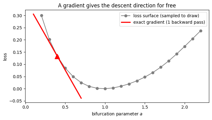
The red tangent is the exact slope at our current guess, computed from a single forward+backward pass. Grid search would need the whole grey curve; evolutionary search would need many scattered samples to estimate that slope. With the gradient in hand, an optimiser steps straight toward the minimum — and the same mechanism scales to thousands of parameters with no extra cost per parameter.

The hands-on version of this fit (with a real optimiser loop) is Fitting with Gradients.

New application scenarios

Differentiability is not just “faster fitting of one knob.” It opens qualitatively new ways of working that grid/evolutionary search cannot reach.

1. Efficient subject-specific fitting

Personalising a whole-brain model to one subject means fitting many local and coupling parameters to that subject’s data. With gradients, a quasi-Newton or Adam optimiser converges in tens of iterations regardless of the parameter count, turning an overnight evolutionary search into minutes. Per-subject fits become routine rather than a compute project.

2. High-dimensional parameter fields

You are no longer restricted to a few global knobs. You can give every region (or every edge) its own parameter — a spatial field of excitability, gain, or coupling — and fit all of them jointly, because the gradient w.r.t. a thousand-dimensional field costs the same backward pass as the gradient w.r.t. one scalar. This is simply infeasible with grid search and painfully sample-hungry for evolutionary methods.

3. Gradient- and Hessian-based identifiability

The gradient (and, via JAX, the Hessian or Fisher information) tells you about the geometry of the loss around an optimum: which parameter combinations are well-constrained by the data and which are sloppy. This is the basis of identifiability and sensitivity analysis — and it falls out of the same autodiff machinery, with no finite-difference noise.

4. Training NMM networks on tasks

Because the rollout is differentiable end-to-end, a network of neural masses can be trained the way a recurrent neural network is — minimise a task loss (classification, working memory, prediction) by gradient descent on the model’s parameters. The model becomes a trainable, biologically-structured RNN. See Training on Tasks for a worked delayed-match-to-sample task.

5. End-to-end differentiable parameters → signal

The forward models (BOLD hemodynamics, EEG/MEG lead fields) are themselves differentiable, so the gradient flows all the way from a neuroimaging-space loss back to the underlying neural parameters. You can fit directly in BOLD or sensor space — parameters → activity → signal → loss — without hand-deriving any sensitivities.

When not to use gradients

Gradients are powerful but not universal, and brainmass is honest about this — the same Fitter exposes gradient-free backends for good reason:

• Non-smooth or phase-degenerate objectives. Matching an oscillatory time series point-by-point has a flat / degenerate gradient (a phase mismatch kills it). Fit a scalar summary — amplitude, functional connectivity, a spectral peak — instead, or fall back to a derivative-free backend.

• Rugged, multi-modal landscapes where you need global exploration: a population-based method (Nevergrad’s differential evolution) may find the basin that gradient descent then refines.

• Discrete or non-differentiable parameters.

brainmass.Fitter lets you write the objective once and switch between backend='grad', 'nevergrad', and 'scipy' — see Gradient-Free Fitting. Differentiability is the default advantage, not a straitjacket.

How brainmass compares

brainmass shares the neural-mass / whole-brain modelling space with The Virtual Brain (TVB) and neurolib. Both are mature, widely-used, and excellent — but both are built on NumPy/Numba, run forward simulations, and fit parameters with grid or evolutionary search. Neither has an automatic- differentiation / JAX core, so neither can backpropagate through the solve or run natively on GPU/TPU.

The table below mirrors the landing-page summary. It is deliberately conservative: “Partial” means a capability exists in some form but is narrower than brainmass’s, and the picture reflects the state of these projects at the time of writing — consult each project for its current status.

Capability	brainmass	The Virtual Brain	neurolib
Differentiable / gradient-based fitting (backprop through the solve)	Yes	No	No
JAX backend with GPU / TPU acceleration	Yes	No	No
In-package orchestration & fitting (Simulator / Network / Fitter)	Yes	Partial	Partial
Unit-safe quantities (dimensional analysis)	Yes	No	No
Next-generation / exact mean-field models (e.g. Montbrió-Pazó-Roxin, Coombes-Byrne)	Yes	Partial	Partial
In-package BOLD + EEG/MEG forward models	Yes	Yes	Partial

A few notes to keep the claims fair:

• TVB and neurolib are not autodiff/JAX frameworks. They are numpy/numba-based. This is a factual statement about backend, not a judgement of quality — TVB in particular has the richest connectome tooling, GUI, and community in the field.

• “In-package forward models.” TVB ships BOLD and EEG/MEG forward models, so it earns a “Yes.” neurolib focuses on BOLD, hence “Partial.”

• “Next-generation mean fields.” All three offer some next-generation models; brainmass derives several (Montbrió-Pazó-Roxin, Coombes-Byrne) exactly from spiking networks, which is the differentiator behind the “Yes.”

The deeper rationale for the JAX-native choice is the whole of this page; the landing page links back here for exactly that reason.

Where to go next

This page is the conceptual hub for the differentiable workflow. The hands-on path through it is:

• Fitting with Gradients — fit a parameter by backprop through the Simulator (the worked version of the example above).

• Gradient-Free Fitting — the same objective with Nevergrad and SciPy backends, head-to-head with gradients.

• Training on Tasks — train a neural-mass network on a task.

• Data-Driven Modeling — the data-driven modelling hub that curates the full differentiable workflow and its roadmap.

And for the conceptual neighbours:

• What Is a Neural Mass Model? — what these models are.

• Architecture Overview — how the differentiable pipeline is built.

References

• Baydin, A. G., Pearlmutter, B. A., Radul, A. A., & Siskind, J. M. (2018). Automatic differentiation in machine learning: a survey. Journal of Machine Learning Research, 18(153), 1–43.

• Bradbury, J., et al. (2018). JAX: composable transformations of Python+NumPy programs. http://github.com/google/jax

• Sanz Leon, P., et al. (2013). The Virtual Brain: a simulator of primate brain network dynamics. Frontiers in Neuroinformatics, 7, 10.

• Cakan, C., Jajcay, N., & Obermayer, K. (2023). neurolib: a simulation framework for whole-brain neural mass modeling. Cognitive Computation, 15, 1132–1152.

• Montbrió, E., Pazó, D., & Roxin, A. (2015). Macroscopic description for networks of spiking neurons. Physical Review X, 5(2), 021028.