Forward Models

A neural-mass model evolves hidden dynamics – firing rates, synaptic gating, membrane potentials. None of those are what an experiment actually records. A forward model (or observation model) is the biophysical map from that hidden activity to a measurable neuroimaging signal:

Neural-mass model  ->  Forward model  ->  Observable signal
(hidden dynamics)      (biophysics)       (BOLD / EEG / MEG)

This is the bridge that turns a simulation into something you can compare against data – the prerequisite for the fitting and training tutorials that follow. In this notebook you will:

1. build a small multi-region source with Network and a bundled connectome,

2. map excitatory activity to fMRI BOLD two ways – the convolution HRFBold and the Balloon–Windkessel BOLDSignal,

3. project a millisecond-scale cortical source to EEG and MEG sensors through unit-aware lead-field operators, and

4. read out and visualise each modality with brainmass.viz.

Note

Every cell runs against the current API. The connectivity and lead-field matrices are small synthetic stand-ins so the page builds fast – swap in your own structural connectome and BEM-derived lead fields for a real study.

import brainmass
import brainstate
import braintools
import brainunit as u
import jax.numpy as jnp
import numpy as np
import matplotlib.pyplot as plt

# A delay-coupled Network sizes its delay buffer from the global dt at construction,
# so set dt once here, before building any Network.
brainstate.environ.set(dt=1.0 * u.ms)
brainstate.random.seed(0)

An NVIDIA GPU may be present on this machine, but a CUDA-enabled jaxlib is not installed. Falling back to cpu.

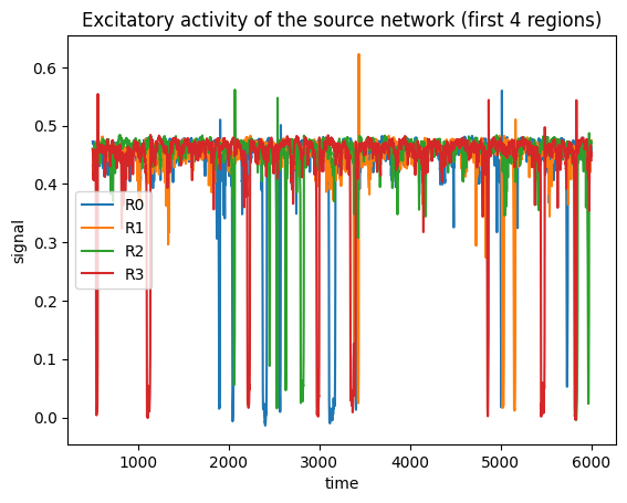
A multi-region source

BOLD and EEG/MEG both observe the activity of many regions, so we first build a small whole-brain source. We load the bundled 8-region example connectome and wire it into a Network of WilsonCowanStep nodes. Per-region Ornstein–Uhlenbeck noise (noise_E=...) gives each region its own fluctuations – without it a deterministic network collapses to one shared fixed point and the observed signals would be perfectly correlated (a degenerate functional connectivity).

conn = brainmass.datasets.load_dataset('example_connectome')
N = conn.weights.shape[0]
labels = list(conn.labels)
print(f"connectome: {N} regions, labels = {labels}")

node = brainmass.WilsonCowanStep(
    in_size=N,
    noise_E=brainmass.OUProcess(N, sigma=0.4, tau=20.0 * u.ms),
)
net = brainmass.Network(
    node,
    conn=conn.weights,
    distance=conn.distances,
    speed=10.0 * u.mm / u.ms,
    coupling='diffusive',
    coupled_var='rE',
    k=0.5,
)

# Run the source network; monitor each region's excitatory rate rE.
src = brainmass.Simulator(net, dt=1.0 * u.ms).run(
    6000.0 * u.ms,
    monitors=lambda m: m.node.rE.value,
    transient=500.0 * u.ms,
)
neural = src['output']          # (T, N) excitatory rate (dimensionless WilsonCowan rate)
ts = src['ts']
print("neural source:", neural.shape, "| unit:", u.get_unit(neural))

ax = brainmass.viz.plot_timeseries(neural[:, :4], ts=ts, labels=labels[:4])
ax.set_title("Excitatory activity of the source network (first 4 regions)")
plt.show()

connectome: 8 regions, labels = [np.str_('R0'), np.str_('R1'), np.str_('R2'), np.str_('R3'), np.str_('R4'), np.str_('R5'), np.str_('R6'), np.str_('R7')]

neural source: (5500, 8) | unit: 1

BOLD: from neural activity to fMRI

The fMRI BOLD signal is the hemodynamic response to neural activity – slow (timescale of seconds) and lagged. brainmass ships two forward models; they trade speed and differentiability against biophysical detail.

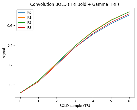
Convolution BOLD (HRFBold)

HRFBold convolves the neural drive with a hemodynamic response function (HRF) kernel and downsamples to the fMRI repetition time (TR). It is a single linear convolution – fast and differentiable in its scalar parameters – which makes it the natural choice when BOLD is the target of a fit. Several closed-form kernels are available (GammaHRFKernel, DoubleExponentialHRFKernel, MixtureOfGammasHRFKernel, …).

hrf = brainmass.HRFBold(
    period=720.0 * u.ms,            # output TR (~0.72 s, a fast multiband protocol)
    downsample_period=20.0 * u.ms,  # internal convolution step
    kernel=brainmass.GammaHRFKernel(),
)
bold_conv = hrf(u.get_magnitude(neural), dt=1.0 * u.ms)   # (T_bold, N), dimensionless
print("HRFBold BOLD:", bold_conv.shape)

ax = brainmass.viz.plot_timeseries(bold_conv[:, :4], labels=labels[:4])
ax.set_xlabel("BOLD sample (TR)")
ax.set_title("Convolution BOLD (HRFBold + Gamma HRF)")
plt.show()

HRFBold BOLD: (7, 8)

Balloon–Windkessel BOLD (BOLDSignal)

BOLDSignal integrates the four-state Balloon–Windkessel ODE (blood volume, flow, deoxyhemoglobin) – the choice when biophysical realism matters. It is dimensionless and its RK2 integrator advances t + dt, so it needs a unitless dt in environ (a Quantity dt would raise on ms + 1). We therefore drive it with dt = 0.01 while the neural stage used 1.0 * u.ms; restore the time-unit dt afterwards.

brainstate.environ.set(dt=0.01)            # dimensionless dt for the haemodynamic ODE
bold_model = brainmass.BOLDSignal(in_size=N)
bold_model.init_all_states()

def bold_step(z):
    bold_model.update(z)
    return bold_model.bold()

bold_balloon = brainstate.transform.for_loop(bold_step, u.get_magnitude(neural))  # (T, N)
brainstate.environ.set(dt=1.0 * u.ms)      # restore the time-unit dt

print("BOLDSignal BOLD:", bold_balloon.shape)

fig, axes = plt.subplots(1, 2, figsize=(11, 3.5))
brainmass.viz.plot_timeseries(bold_conv[:, 0], ax=axes[0])
axes[0].set_title("Convolution BOLD (region R0)")
axes[0].set_xlabel("TR")
brainmass.viz.plot_timeseries(bold_balloon[::50, 0], ax=axes[1])
axes[1].set_title("Balloon-Windkessel BOLD (region R0)")
axes[1].set_xlabel("downsampled step")
plt.tight_layout()
plt.show()

BOLDSignal BOLD: (5500, 8)

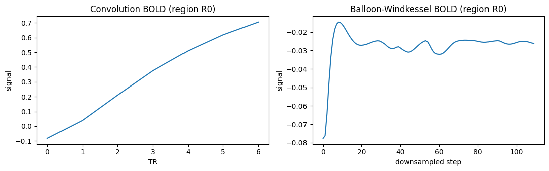
Both BOLD pipelines track the same slow envelope of the neural drive; they differ in their intrinsic hemodynamic latency, so compare BOLD waveforms over a small lag rather than at exact zero lag. Use HRFBold for fast, differentiable fitting and BOLDSignal when you need the full Balloon–Windkessel biophysics.

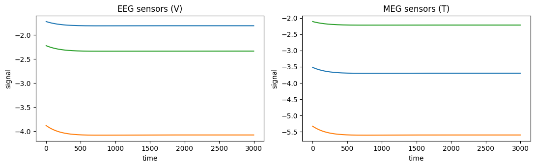
EEG and MEG: lead-field forward models

EEG and MEG are instantaneous linear projections of cortical dipole activity onto sensors. The lead field L is the gain matrix that maps each region’s dipole moment to each sensor. brainmass provides unit-aware operators that carry the physics:

• EEGLeadFieldModel – scalp potentials in volts,

• MEGLeadFieldModel / LeadFieldModel – magnetic fields in tesla.

We use a JansenRitStep source whose pyramidal observable (jr.eeg(), the classic EEG correlate) is a millisecond-scale membrane potential in mV – exactly the kind of fast signal EEG/MEG record.

R, M = 4, 6   # 4 cortical sources, 6 sensors

jr = brainmass.JansenRitStep(in_size=R)
eeg_src = brainmass.Simulator(jr, dt=0.1 * u.ms).run(
    400.0 * u.ms,
    monitors=lambda m: m.eeg(),     # pyramidal observable, shape (T, R), in mV
    transient=100.0 * u.ms,
)['output']
print("Jansen-Rit source:", eeg_src.shape, "| unit:", u.get_unit(eeg_src))

rng = np.random.RandomState(1)

# EEG lead field: gain in volt / (nA*m); the helper assumes an mV source.
L_eeg = jnp.asarray(rng.rand(R, M)) * (u.volt / (u.nA * u.meter))
eeg_model = brainmass.EEGLeadFieldModel(in_size=(R,), out_size=(M,), L=L_eeg, sensor_unit=u.volt)
eeg = eeg_model.update(eeg_src)     # (T, M) in volts

# MEG lead field: gain in tesla / (nA*m). We use the base LeadFieldModel with an explicit
# `scale` so the mV source is converted to a dipole moment before projection.
L_meg = jnp.asarray(rng.rand(R, M)) * (u.tesla / (u.nA * u.meter))
meg_model = brainmass.LeadFieldModel(
    in_size=(R,), out_size=(M,), L=L_meg,
    sensor_unit=u.tesla, dipole_unit=u.nA * u.meter, scale=u.nA * u.meter / u.mV,
)
meg = meg_model.update(eeg_src)     # (T, M) in tesla

print("EEG sensors:", eeg.shape, "| unit:", u.get_unit(eeg))
print("MEG sensors:", meg.shape, "| unit:", u.get_unit(meg))

Jansen-Rit source: (3000, 4) | unit: mV
EEG sensors: (3000, 6) | unit: V
MEG sensors: (3000, 6) | unit: T

fig, axes = plt.subplots(1, 2, figsize=(11, 3.5))
brainmass.viz.plot_timeseries(eeg[:, :3], ax=axes[0])
axes[0].set_title("EEG sensors (V)")
brainmass.viz.plot_timeseries(meg[:, :3], ax=axes[1])
axes[1].set_title("MEG sensors (T)")
plt.tight_layout()
plt.show()

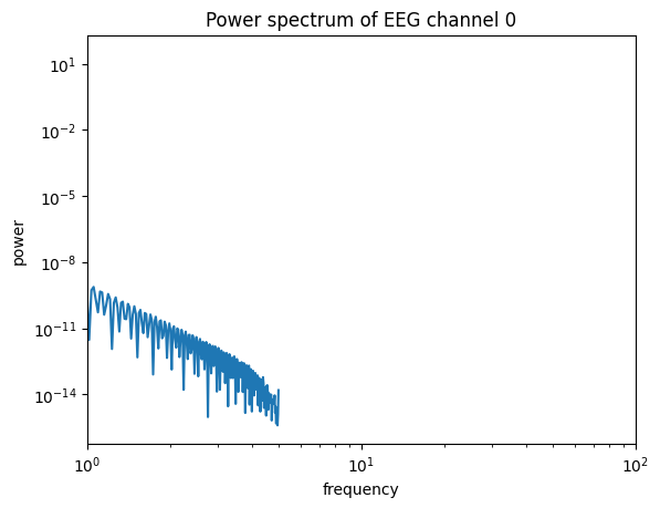
Inspecting the spectrum

A forward model preserves the temporal structure of its source. Estimating the power spectrum of one EEG channel confirms the signal carries the source’s oscillatory content (the Jansen–Rit alpha rhythm). The Jansen–Rit stage used dt = 0.1 ms, i.e. a 10 kHz sampling rate.

ax = brainmass.viz.plot_power_spectrum(eeg[:, 0], dt=0.1 * u.ms)
ax.set_title("Power spectrum of EEG channel 0")
ax.set_xlim(1, 100)
plt.show()

Validating against data: functional connectivity

A common way to score a whole-brain model is the agreement between its functional connectivity (FC, the region x region correlation of the observed signal) and an empirical FC. We compute the BOLD FC from the convolution pipeline and compare it to the FC bundled with the example signal dataset, using the same correlation that brainmass.objectives will optimise in the next tutorial.

sig = brainmass.datasets.load_dataset('example_signal')
fc_target = sig.fc                                  # (N, N) "empirical" FC

fc_corr = brainmass.objectives.fc_corr()            # builder -> callable(pred, target)
score = float(fc_corr(bold_conv, fc_target))        # Pearson corr between the two FC matrices
print(f"FC(simulated BOLD) vs FC(empirical): correlation = {score:.3f}")

fig, axes = plt.subplots(1, 2, figsize=(9, 4))
brainmass.viz.plot_functional_connectivity(bold_conv, labels=labels, ax=axes[0])
axes[0].set_title("Simulated BOLD FC")
brainmass.viz.plot_functional_connectivity(fc_target, is_matrix=True, labels=labels, ax=axes[1])
axes[1].set_title("Empirical FC (target)")
plt.tight_layout()
plt.show()

FC(simulated BOLD) vs FC(empirical): correlation = 0.101

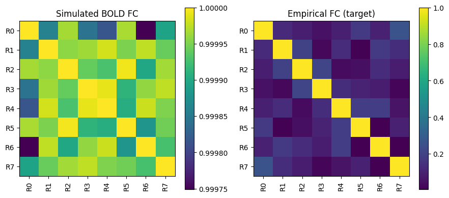
That single scalar – the FC correlation – is exactly the kind of summary objective the fitter minimises. Driving it up by adjusting model parameters is the subject of the next tutorial.

Summary

• A forward model maps hidden neural dynamics to an observable signal.

• HRFBold (fast, differentiable convolution) and BOLDSignal (Balloon–Windkessel ODE) both turn neural activity into BOLD; pick the former for fitting, the latter for biophysical realism.

• EEGLeadFieldModel and LeadFieldModel project a cortical source to EEG (volts) and MEG (tesla) through a unit-aware lead field.

• brainmass.objectives turns a prediction-vs-data comparison (e.g. FC correlation) into a single scalar – the bridge to fitting.

Next steps

• Fitting with Gradients – fit model parameters to an observed signal by backpropagating through the solve.

• Gradient-Free Fitting – the same fit with gradient-free search.

• Forward Models – complete forward-model and lead-field API.

• Observation Models – HRF kernels and observation models.