Training a HORN Network on a Cognitive Task

The previous case studies fit a few biophysical parameters. This one trains an entire recurrent network — every weight — to perform a task, the data-driven showcase of a differentiable brain model. Because brainmass networks are end-to-end differentiable, the same backpropagation that fit one parameter scales to training a recurrent network with gradient descent.

We train a HORNSeqNetwork — a recurrent network of coupled harmonic oscillators (a Harmonic Oscillator Recurrent Network) — on the bundled delayed match-to-sample task. The network sees a cue symbol, must hold it across a delay, then sees a probe and decides whether they match. Solving it requires genuine working memory in the recurrent dynamics.

Source: consolidates the HORN cognitive-task training scripts onto the bundled brainmass.datasets.delayed_match_task() — fully self-contained, no downloads.

Note

Fitter targets parameter fitting against a single fixed target. Task training — minibatched (inputs, targets) over epochs with a held-out metric — is a different loop, so we drive a braintools.optim optimizer directly. A future Trainer would wrap this loop.

1. The task

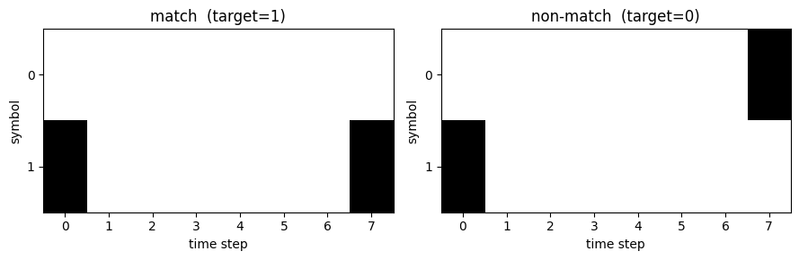
brainmass.datasets.delayed_match_task() synthesises the dataset. Each trial is a sequence: a one-hot cue symbol at the first step, blank steps (the delay), then a one-hot probe at the last step. The binary target is 1 if probe matches cue, else 0. We use a 2-symbol alphabet and 8-step sequences, and hold out a test split.

inputs_np, targets_np = brainmass.datasets.delayed_match_task(
    n_samples=320, seq_len=8, n_symbols=2, seed=0,
)
print("inputs :", inputs_np.shape, "(n_samples, seq_len, n_symbols)")
print("targets:", targets_np.shape, " class balance =", f"{targets_np.mean():.2f}")

inputs = jnp.asarray(inputs_np, dtype=jnp.float32)
targets = jnp.asarray(targets_np, dtype=jnp.int32)
n_train = 256
X_train, y_train = inputs[:n_train], targets[:n_train]
X_test, y_test = inputs[n_train:], targets[n_train:]
n_symbols = inputs.shape[2]

fig, axes = plt.subplots(1, 2, figsize=(9, 3))
for ax, idx, name in [(axes[0], int(np.argmax(targets_np == 1)), 'match'),
                      (axes[1], int(np.argmax(targets_np == 0)), 'non-match')]:
    ax.imshow(inputs_np[idx].T, aspect='auto', cmap='Greys', interpolation='nearest')
    ax.set_title(f'{name}  (target={int(targets_np[idx])})')
    ax.set_xlabel('time step'); ax.set_ylabel('symbol'); ax.set_yticks(range(n_symbols))
plt.tight_layout()
plt.show()

inputs : (320, 8, 2) (n_samples, seq_len, n_symbols)
targets: (320,)  class balance = 0.50

2. The HORN classifier

A HORNSeqNetwork maps an input sequence (T, n_input) to one output vector by running its oscillator dynamics over the sequence and reading out the final state. We give it two output units (match / non-match logits) and raise the oscillator excitability alpha above its default so it responds strongly enough to learn quickly.

The network writes its hidden states in place, and init_state allocates them unbatched. To process a mini-batch we reset the hidden states to the batch shape before each forward pass and feed the sequence as (T, batch, n_input) (time leading).

net = brainmass.HORNSeqNetwork(
    n_input=n_symbols,
    n_hidden=64,
    n_output=2,
    alpha=0.2,                 # excitability (raised from the 0.04 default)
    omega=2 * np.pi / 28,
)
brainstate.nn.init_all_states(net)

def reset_hidden(batch_size):
    # HORN allocates hidden states unbatched; broadcast them to the batch shape.
    for layer in net.layers:
        shape = (batch_size,) + tuple(layer.horn.in_size)
        layer.horn.x.value = jnp.zeros(shape)
        layer.horn.y.value = jnp.zeros(shape)

def logits(batch_inputs):                       # (B, T, n_symbols) -> (B, 2)
    reset_hidden(batch_inputs.shape[0])
    seq = jnp.transpose(batch_inputs, (1, 0, 2))  # (T, B, n_symbols): time leads
    return net(seq)

weights = net.states(brainstate.ParamState)
print("trainable weight tensors:", len(weights))

trainable weight tensors: 3

3. The training loop

The loss is softmax cross-entropy between the logits and the binary target, with accuracy tracked alongside. We register the trainable weights with Adam and, each step, take the gradient of the loss through the whole recurrent rollout (brainstate.transform.grad()) and apply it — the canonical brainmass training primitive, jitted for speed. The only new ingredients beyond the fitting case study are minibatching and the epoch loop.

optimizer = braintools.optim.Adam(lr=3e-2)
optimizer.register_trainable_weights(weights)

def loss_and_acc(batch_inputs, batch_targets):
    lg = logits(batch_inputs)
    logp = jax.nn.log_softmax(lg, axis=-1)
    ce = -jnp.mean(logp[jnp.arange(batch_targets.shape[0]), batch_targets])
    acc = jnp.mean(jnp.argmax(lg, axis=-1) == batch_targets)
    return ce, acc

@brainstate.transform.jit
def train_step(batch_inputs, batch_targets):
    grad_fn = brainstate.transform.grad(
        lambda: loss_and_acc(batch_inputs, batch_targets),
        weights, has_aux=True, return_value=True,
    )
    grads, loss, acc = grad_fn()
    optimizer.step(grads)
    return loss, acc

@brainstate.transform.jit
def evaluate(batch_inputs, batch_targets):
    return loss_and_acc(batch_inputs, batch_targets)

n_epochs, batch_size = 20, 32
history = {'epoch': [], 'train_loss': [], 'train_acc': [], 'test_acc': []}
for epoch in range(n_epochs):
    perm = np.random.RandomState(epoch).permutation(n_train)
    losses, accs = [], []
    for start in range(0, n_train, batch_size):
        idx = perm[start:start + batch_size]
        if len(idx) < batch_size:
            continue
        loss, acc = train_step(X_train[idx], y_train[idx])
        losses.append(float(loss)); accs.append(float(acc))
    _, test_acc = evaluate(X_test, y_test)
    history['epoch'].append(epoch)
    history['train_loss'].append(float(np.mean(losses)))
    history['train_acc'].append(float(np.mean(accs)))
    history['test_acc'].append(float(test_acc))
    if epoch % 4 == 0 or epoch == n_epochs - 1:
        print(f"epoch {epoch:2d}: train_loss={np.mean(losses):.4f} "
              f"train_acc={np.mean(accs):.3f}  test_acc={float(test_acc):.3f}")

epoch  0: train_loss=1.1386 train_acc=0.543  test_acc=0.516

epoch  4: train_loss=0.6885 train_acc=0.562  test_acc=0.516

epoch  8: train_loss=0.6811 train_acc=0.676  test_acc=0.750

epoch 12: train_loss=0.5739 train_acc=0.785  test_acc=1.000

epoch 16: train_loss=0.2497 train_acc=1.000  test_acc=1.000

epoch 19: train_loss=0.1423 train_acc=1.000  test_acc=1.000

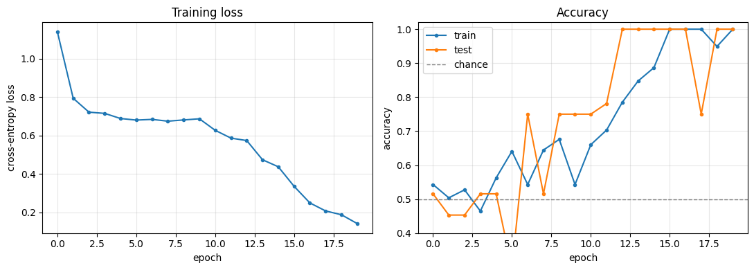
4. Results

The network starts at chance (~50%, a binary task) and — as gradient descent shapes its recurrent weights to hold the cue across the delay — climbs toward perfect accuracy on both the training and the held-out test set.

final_train = history['train_acc'][-1]
final_test = history['test_acc'][-1]
print(f"final train accuracy: {final_train:.1%}")
print(f"final test  accuracy: {final_test:.1%}")

fig, (ax1, ax2) = plt.subplots(1, 2, figsize=(11, 4))
ax1.plot(history['epoch'], history['train_loss'], marker='.')
ax1.set_xlabel('epoch'); ax1.set_ylabel('cross-entropy loss')
ax1.set_title('Training loss'); ax1.grid(alpha=0.3)
ax2.plot(history['epoch'], history['train_acc'], marker='.', label='train')
ax2.plot(history['epoch'], history['test_acc'], marker='.', label='test')
ax2.axhline(0.5, color='grey', ls='--', lw=1, label='chance')
ax2.set_xlabel('epoch'); ax2.set_ylabel('accuracy')
ax2.set_ylim(0.4, 1.02); ax2.set_title('Accuracy'); ax2.legend(); ax2.grid(alpha=0.3)
plt.tight_layout()
plt.show()

final train accuracy: 100.0%
final test  accuracy: 100.0%

Summary

We trained a recurrent harmonic-oscillator network to perform a working-memory task:

• the bundled delayed_match_task() provides minibatchable (inputs, targets) — no external download,

• a HORNSeqNetwork reads a sequence to a decision, with hidden states reset to the batch shape each forward pass,

• gradient descent through the full recurrent rollout (jitted brainstate.transform.grad + braintools.optim.Adam) drives accuracy from chance to near-perfect on a held-out split.

This is the differentiable-brain showcase: the same autodiff that fits a single coupling strength trains an entire network end to end. The one piece Fitter does not yet own — minibatched task training with a held-out metric — is the loop a future Trainer would wrap.