Compose a Custom Objective

Compose a Custom Objective#

Goal: build the loss your fit actually needs — combine the brainmass.objectives builders, write your own, and plug the result into brainmass.Fitter.

An objective in brainmass is a small callable(prediction, target) -> scalar that is jit / grad / vmap-safe and unit-aware. The builders in brainmass.objectives return such callables; you compose them or write your own with the same signature.

The built-in toolkit#

Every entry in brainmass.objectives is a builder that returns a loss/score callable. They wrap braintools.metric — no metric maths is reimplemented.

import numpy as np
rng = np.random.default_rng(0)
pred = jnp.asarray(rng.standard_normal((200, 6)))    # (time, regions)
target = jnp.asarray(rng.standard_normal((200, 6)))

print("timeseries_rmse :", float(objectives.timeseries_rmse()(pred, target)))
print("fc_corr (score) :", float(objectives.fc_corr()(pred, target)))
print("fc_corr (loss)  :", float(objectives.fc_corr(as_loss=True)(pred, target)))
print("cosine_sim      :", float(objectives.cosine_sim()(pred, target)))
print("fcd (loss)      :", float(objectives.fcd(as_loss=True)(pred, target)))

timeseries_rmse : 1.433825135231018

fc_corr (score) : -0.19663743674755096
fc_corr (loss)  : 1.1966373920440674

cosine_sim      : -0.025183098390698433

fcd (loss)      : 0.5260788798332214

A few conventions worth knowing:

Score vs loss. fc_corr / cosine_sim / fcd return a score to maximise by default; pass as_loss=True to get 1 - score, a quantity to minimise. timeseries_rmse / fc_rmse are already losses.
Unit safety. timeseries_rmse subtracts before stripping units, so mixing mV and Hz raises. FC / cosine objectives are scale-invariant and operate on magnitudes.
Identity is exact. Every loss returns 0 (and every score 1) when prediction equals target.

x = jnp.zeros((50, 4)) + jnp.asarray(rng.standard_normal((50, 4)))
print("rmse(x, x)    =", float(objectives.timeseries_rmse()(x, x)))
print("fc_corr(x, x) =", float(objectives.fc_corr()(x, x)))

rmse(x, x)    = 0.0

fc_corr(x, x) = 1.0

Combine weighted objectives#

objectives.combine sums (weight, objective) pairs into one callable — the standard way to balance, say, a time-domain term against a connectivity term.

combined = objectives.combine(
    (1.0, objectives.timeseries_rmse()),
    (0.5, objectives.fc_corr(as_loss=True)),
)
print("combined loss:", float(combined(pred, target)))

# Sanity check the arithmetic on a controlled example:
a = jnp.zeros((10, 3))
check = objectives.combine(
    (2.0, objectives.timeseries_rmse()),
    (0.5, objectives.timeseries_rmse()),
)
print("(2.0 + 0.5) * 1.0 =", float(check(a + 1.0, a)))

combined loss: 2.0321438312530518

(2.0 + 0.5) * 1.0 = 2.5

Write your own objective#

A custom objective is any function with the (prediction, target) -> scalar signature, built from jax.numpy so it stays differentiable. Two rules:

Reduce to a scalar (a gradient optimiser needs one number).
Strip units with u.get_magnitude only where the quantity is scale-free; keep them through a subtraction so unit mismatches are caught.

Here is a spectral-peak objective: match the dominant oscillation frequency of each region. It reuses braintools.metric.power_spectral_density rather than hand-rolling an FFT. (power_spectral_density(signal, dt_ms) returns frequencies in cycles per dt unit; comparing two peaks in the same units is all we need.)

def peak_frequency_mse(dt_ms=1.0):
    """Loss matching the dominant spectral peak of each region."""
    def loss(prediction, target):
        def peak_freqs(sig):
            sig = u.get_magnitude(sig)
            def one(col):
                freqs, psd = braintools.metric.power_spectral_density(col, dt_ms)
                return freqs[jnp.argmax(psd)]
            return jax.vmap(one, in_axes=1)(sig)  # (regions,)
        diff = peak_freqs(prediction) - peak_freqs(target)
        return jnp.mean(diff ** 2)
    return loss

# A 4-region bank of sinusoids at well-separated frequencies, sampled at 1 ms.
samples = np.arange(1000)
dt_s = 1e-3  # 1 ms sampling
rng2 = np.random.default_rng(1)
def sine_bank(freqs_hz):
    cols = [np.sin(2 * np.pi * f * samples * dt_s) + 0.05 * rng2.standard_normal(1000)
            for f in freqs_hz]
    return jnp.asarray(np.stack(cols, axis=1))

pred_sig = sine_bank([5, 10, 20, 30])
fast_sig = sine_bank([8, 16, 28, 40])

spec_loss = peak_frequency_mse(dt_ms=1.0)
print("peak-freq loss (pred vs fast):", float(spec_loss(pred_sig, fast_sig)))
print("peak-freq loss (pred vs pred):", float(spec_loss(pred_sig, pred_sig)))

peak-freq loss (pred vs fast): 6.103515625e-05
peak-freq loss (pred vs pred): 0.0

Custom objectives compose with the built-ins through combine, exactly like the library ones — they share the same signature. Here a connectivity term and the spectral term are balanced into one loss (both inputs have ≥2 regions, so fc_corr is well-defined).

mixed = objectives.combine(
    (1.0, objectives.fc_corr(as_loss=True)),
    (0.1, peak_frequency_mse(dt_ms=1.0)),
)
print("mixed FC + spectral loss:", float(mixed(pred_sig, fast_sig)))

mixed FC + spectral loss: 1.7818667888641357

Plug an objective into `Fitter`#

brainmass.Fitter accepts an objective two ways:

objective= — a (prediction, target) callable; the Fitter builds the loss as objective(predict(model), target) + model.reg_loss(), and you supply predict (a Simulator closure) and the target.
loss_fn= — a full loss_fn(model) -> (scalar, aux) that you own entirely, for losses against a derived scalar summary (the right choice for oscillators, where a point-by-point timeseries_rmse is phase-degenerate).

Here we fit the Hopf bifurcation parameter a so the settled amplitude matches a target, using a custom scalar objective inside loss_fn.

def amplitude_loss(target_amp):
    def loss(prediction):
        x = u.get_magnitude(prediction)
        amp = jnp.sqrt(jnp.mean(x ** 2)) * jnp.sqrt(2.0)
        return (amp - target_amp) ** 2, amp
    return loss

target_amp = 1.2
obj = amplitude_loss(target_amp)

# Mark `a` trainable with a Param; a plain Param(fit=True) lives in physical space.
node = brainmass.HopfStep(in_size=1, a=Param(0.1, fit=True), w=0.3,
                          init_x=braintools.init.Constant(0.5))

def loss_fn(m):
    res = brainmass.Simulator(m, dt=0.1 * u.ms).run(
        150 * u.ms, monitors=['x'], transient=50 * u.ms)
    return obj(res['x'])   # (scalar loss, amplitude aux)

fitter = brainmass.Fitter(node, braintools.optim.Adam(lr=0.05), loss_fn=loss_fn)
result = fitter.fit(n_steps=40)
print(f"target amplitude : {target_amp}")
print(f"fitted a         : {result.best_params['a']:.3f}")
print(f"best loss        : {result.best_loss:.2e}")

target amplitude : 1.2
fitted a         : 1.232
best loss        : 8.41e-03

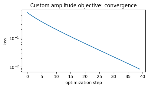
The fit drives a from 0.1 toward the value whose limit cycle has amplitude 1.2. Plot the loss curve from result.history:

hist = np.asarray(result.history)
fig, ax = plt.subplots(figsize=(5, 3))
ax.semilogy(hist)
ax.set_xlabel('optimization step')
ax.set_ylabel('loss')
ax.set_title('Custom amplitude objective: convergence')
fig.tight_layout()
plt.show()

../_images/dd611bdfd6a3ec1b6c3a68cda90a03fe3b1b6cfe178f17551e72af311c35dfb3.png

Using `objective=` with a `predict` closure#

When the loss is a brainmass.objectives builder over the trajectory (e.g. an FC fit), pass it via objective= and supply predict + target. The Fitter handles the reg_loss and the optimisation loop.

# 3-region drive so FC is non-degenerate.
conn = brainmass.datasets.load_dataset('example_connectome')
W3, D3 = conn.weights[:3, :3], conn.distances[:3, :3]
brainstate.environ.set(dt=0.1 * u.ms)

def make_net(k):
    base = brainmass.HopfStep(in_size=3, a=0.3, w=0.3,
                              init_x=braintools.init.Constant(0.3))
    return brainmass.Network(base, conn=W3, distance=D3, speed=10 * u.mm / u.ms,
                             coupling='diffusive', coupled_var='x', k=k)

def simulate(net):
    res = brainmass.Simulator(net, dt=0.1 * u.ms).run(
        400 * u.ms, monitors=lambda m: m.node.x.value, transient=100 * u.ms)
    return res['output']

# Target FC from a "ground-truth" coupling of 1.0.
target_signal = simulate(make_net(1.0))

# Fit k with a trainable Param, FC-correlation objective.
net = make_net(Param(0.3, fit=True))
fitter = brainmass.Fitter(
    net, braintools.optim.Adam(lr=0.05),
    objective=objectives.fc_corr(as_loss=True),
    predict=simulate,
)
res = fitter.fit(target=target_signal, n_steps=30)
print(f"fitted coupling k : {res.best_params['coupling.k']:.3f}  (true 1.0)")
print(f"best FC loss      : {res.best_loss:.4f}")

fitted coupling k : 0.456  (true 1.0)
best FC loss      : 0.0002

Recap#

Objectives are (prediction, target) -> scalar callables; the builders in brainmass.objectives produce them, and combine weights them together.
Write your own with jax.numpy, reduce to a scalar, and keep units through subtractions.
Feed the Fitter a derived-scalar loss_fn= (oscillator amplitude / spectrum) or an objective= + predict= (FC / FCD over the trajectory).

Next steps#

Fitting with Gradients — the full gradient-fitting workflow.
Gradient-Free Fitting — the same objective, derivative-free.
Analyze Results (FC / FCD / spectra) — the metrics these objectives are built on.
Orchestration — the Fitter / objectives API.

Compose a Custom Objective

Contents

Compose a Custom Objective#

The built-in toolkit#

Combine weighted objectives#

Write your own objective#

Plug an objective into `Fitter`#

Using `objective=` with a `predict` closure#

Recap#

Next steps#

Modeling

Infrastructure

Compilation

Compose a Custom Objective

Contents

Compose a Custom Objective#

The built-in toolkit#

Combine weighted objectives#

Write your own objective#

Plug an objective into Fitter#

Using objective= with a predict closure#

Recap#

Next steps#

Plug an objective into `Fitter`#

Using `objective=` with a `predict` closure#