Firing Rates and Population Synchrony

This tutorial covers the population-level measures of braintools.analysis, applied to synthetic data whose ground truth is known. Spike-matrix measures live in braintools.analysis.spike and measures of continuous signals in braintools.analysis.population:

Function	Input	Output
spike.firing_rate(spikes, width, dt)	spike matrix (T, N)	population rate in Hz, smoothed with a box of width width
spike.cross_correlation(spikes, bin, dt)	spike matrix	Wang-Buzsaki coherence \(\kappa\), averaged over pairs
population.voltage_fluctuation(potentials)	membrane potentials (T, N)	Golomb synchrony \(\chi^2 \in [0, 1]\)
population.functional_connectivity(activities)	signals (T, N)	(N, N) Pearson correlation matrix
population.functional_connectivity_dynamics(activities, window_size, step_size)	signals	correlation between sliding-window FC matrices

Time units. Pass times as brainunit quantities (10 * u.ms) and they are converted. Plain numbers follow each function’s documented convention: firing_rate treats them as seconds, cross_correlation as milliseconds. Using quantities avoids having to remember which.

1. Setup and Synthetic Populations

import brainunit as u
import jax.numpy as jnp
import matplotlib.pyplot as plt
import numpy as np

import braintools.analysis as ba

rng = np.random.default_rng(0)
dt = 0.1 * u.ms
T = 20_000  # 2 s
t_ms = np.arange(T) * 0.1

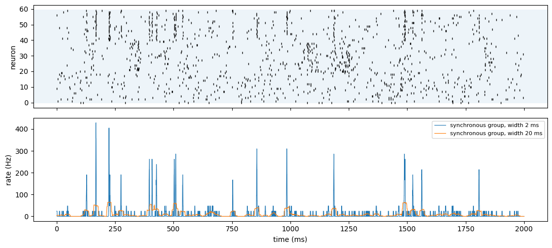
Three groups of 20 neurons, all firing at about 10 Hz on average:

• independent: homogeneous Poisson trains;

• common input: each neuron’s rate is modulated by the same slow signal, so the trains are correlated on a 50 ms time scale but not precisely synchronized;

• synchronous events: background Poisson spikes plus 20 population events in which each neuron fires with probability 0.5 within about 1 ms.

def poisson(rate_hz, shape):
    return (rng.random(shape) < rate_hz * 1e-4).astype(float)  # dt = 0.1 ms


independent = poisson(10.0, (T, 20))

shared = np.convolve(rng.normal(size=T), np.ones(500) / np.sqrt(500), mode="same")  # ~50 ms correlated
modulation = np.exp(1.2 * shared)
rate = 10.0 * modulation / modulation.mean()  # mean exactly 10 Hz
common = (rng.random((T, 20)) < (rate * 1e-4)[:, None]).astype(float)

events = rng.choice(np.arange(500, T - 500), 20, replace=False)
synchronous = poisson(5.0, (T, 20))
for e in events:
    fire = rng.random(20) < 0.5
    synchronous[e + rng.integers(-10, 11, fire.sum()), np.flatnonzero(fire)] = 1

spikes = np.concatenate([independent, common, synchronous], axis=1)
groups = {"independent": slice(0, 20), "common input": slice(20, 40), "synchronous": slice(40, 60)}
for name, g in groups.items():
    print(f"{name:13s} mean rate {spikes[:, g].sum() / 20 / 2.0:5.1f} Hz")

independent   mean rate  10.4 Hz
common input  mean rate   9.7 Hz
synchronous   mean rate  10.4 Hz

2. Raster Plot and Population Rate

For a raster, np.nonzero on the spike matrix gives the time step and neuron index of every spike (the deprecated braintools.metric.raster_plot did the same; braintools.spike.SpikeTrains replaces it). firing_rate averages the spike matrix over neurons and smooths it with a box of width width, giving the population rate in Hz; a wider box trades temporal detail for less noise.

t_idx, idx = np.nonzero(spikes)  # time step and neuron of every spike
times = t_ms[t_idx]
print(f"{len(times)} spikes, neuron indices {int(idx.min())}..{int(idx.max())}")

fig, axes = plt.subplots(2, 1, figsize=(11, 5), sharex=True)
axes[0].plot(times, idx, "|", ms=3, color="k")
for name, g in groups.items():
    axes[0].axhspan(g.start - 0.5, g.stop - 0.5, alpha=0.08)
axes[0].set_ylabel("neuron")
for width in [2 * u.ms, 20 * u.ms]:
    r = ba.spike.firing_rate(spikes[:, 40:60], width, dt)
    axes[1].plot(t_ms, r, lw=0.8, label=f"synchronous group, width {width}")
axes[1].set_ylabel("rate (Hz)")
axes[1].set_xlabel("time (ms)")
axes[1].legend(fontsize=8)
fig.tight_layout()
plt.show()

r = ba.spike.firing_rate(spikes[:, :20], 20 * u.ms, dt)
print(f"independent group: time-averaged rate {float(r.mean()):.2f} Hz (spike count gives "
      f"{spikes[:, :20].sum() / 20 / 2.0:.2f} Hz)")
print("same result with seconds:", float(ba.spike.firing_rate(spikes[:, :20], 0.02 * u.second, 1e-4 * u.second).mean()))

1219 spikes, neuron indices 0..59

independent group: time-averaged rate 10.34 Hz (spike count gives 10.38 Hz)
same result with seconds: 10.343284606933594

3. Spike-Count Coherence \(\kappa\) (cross_correlation)

The spike trains are cut into bins of width bin; \(X_i(l) \in \{0, 1\}\) marks whether neuron \(i\) fired in bin \(l\), and for each pair

\[\kappa_{ij} = \frac{\sum_l X_i(l) X_j(l)}{\sqrt{\sum_l X_i(l) \sum_l X_j(l)}},\]

averaged over all pairs (Wang & Buzsaki, 1996). \(\kappa\) is not corrected for chance: for independent trains, \(\kappa\) is roughly the probability that a bin contains a spike, so it grows with firing rate and bin width. Always compare against a chance level, for example obtained by circularly shifting each train by a random amount, which keeps rates and spike patterns but destroys their alignment.

def shuffled(s):
    return np.stack([np.roll(s[:, i], rng.integers(T)) for i in range(s.shape[1])], axis=1)


print(f"{'group':13s} {'kappa':>7s} {'shuffled':>9s}   (bin = 5 ms)")
for name, g in groups.items():
    k = float(ba.spike.cross_correlation(spikes[:, g], 5 * u.ms, dt))
    k0 = float(ba.spike.cross_correlation(shuffled(spikes[:, g]), 5 * u.ms, dt))
    print(f"{name:13s} {k:7.3f} {k0:9.3f}")

print("\nindependent Poisson trains: kappa grows with rate")
for rate_hz in [5, 20, 80]:
    k = float(ba.spike.cross_correlation(poisson(rate_hz, (T, 20)), 5 * u.ms, dt))
    print(f"  {rate_hz:3d} Hz: kappa {k:.3f}, P(spike in a 5 ms bin) = {1 - np.exp(-rate_hz * 0.005):.3f}")

group           kappa  shuffled   (bin = 5 ms)

independent     0.056     0.053
common input    0.103     0.043
synchronous     0.272     0.045

independent Poisson trains: kappa grows with rate

    5 Hz: kappa 0.023, P(spike in a 5 ms bin) = 0.025
   20 Hz: kappa 0.095, P(spike in a 5 ms bin) = 0.095
   80 Hz: kappa 0.330, P(spike in a 5 ms bin) = 0.330

The synchronous group stands far above its shuffled level, and the common-input group is above it as well. The independent group is at chance, whose value depends on the rate. A raw \(\kappa\) is only interpretable next to its chance level.

4. Membrane-Potential Synchrony \(\chi^2\) (voltage_fluctuation)

For membrane potentials \(V_i(t)\) and their population average \(\bar V(t)\), Golomb’s measure is

\[\chi^2 = \frac{\operatorname{Var}_t[\bar V]}{\frac1N\sum_i \operatorname{Var}_t[V_i]} \in [0, 1],\]

equal to 1 for identical traces and about \(1/N\) for independent ones. If every trace is a shared signal with variance fraction \(c\) plus independent noise, \(\chi^2 \approx c + (1 - c)/N\).

N = 40
n_t = 5000
common_v = rng.normal(size=n_t)
print(f"{'shared fraction c':>18s} {'chi^2':>7s} {'c + (1-c)/N':>12s}")
for c in [0.0, 0.2, 0.5, 0.9, 1.0]:
    V = np.sqrt(c) * common_v[:, None] + np.sqrt(1 - c) * rng.normal(size=(n_t, N))
    print(f"{c:18.1f} {float(ba.population.voltage_fluctuation(V)):7.3f} {c + (1 - c) / N:12.3f}")

 shared fraction c   chi^2  c + (1-c)/N

               0.0   0.025        0.025

               0.2   0.215        0.220
               0.5   0.508        0.512
               0.9   0.901        0.902

               1.0   1.000        1.000

5. Functional Connectivity

functional_connectivity is the Pearson correlation matrix of the columns of its input (np.corrcoef of the transposed array). For spikes, bin them first; the bin width sets the time scale of the correlations you detect. With 50 ms bins both correlated groups stand out from the independent one, which sits near zero.

counts = spikes.reshape(-1, 500, 60).sum(axis=1)  # 50 ms bins
fc = np.asarray(ba.population.functional_connectivity(counts))
print("matches np.corrcoef:", np.allclose(fc, np.corrcoef(counts.T), atol=1e-5))

fig, ax = plt.subplots(figsize=(4.5, 4))
im = ax.imshow(fc, cmap="RdBu_r", vmin=-1, vmax=1)
ax.set_title("FC of 50 ms spike counts")
fig.colorbar(im, ax=ax)
plt.show()

off = ~np.eye(20, dtype=bool)
for name, g in groups.items():
    print(f"{name:13s} mean within-group correlation {fc[g, g][off].mean():+.3f}")

matches np.corrcoef: True

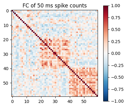
independent   mean within-group correlation +0.038
common input  mean within-group correlation +0.259
synchronous   mean within-group correlation +0.286

functional_connectivity_dynamics slides a window along the signals, computes an FC matrix in each window, and correlates the FC matrices with each other. Blocks in the resulting matrix are periods with a stable connectivity pattern. Below, 8 signals switch halfway from one correlation structure (channels 0-3 coupled) to another (channels 4-7 coupled).

n_t = 4000
x = rng.normal(size=(n_t, 8))
drive = rng.normal(size=n_t)
x[: n_t // 2, :4] += 1.5 * drive[: n_t // 2, None]
x[n_t // 2:, 4:] += 1.5 * drive[n_t // 2:, None]

fcd = np.asarray(ba.population.functional_connectivity_dynamics(x, window_size=200, step_size=50))
fig, ax = plt.subplots(figsize=(4, 3.5))
im = ax.imshow(fcd, cmap="viridis")
ax.set_xlabel("window")
ax.set_ylabel("window")
fig.colorbar(im, ax=ax)
plt.show()
h = fcd.shape[0] // 2
print(f"{fcd.shape[0]} windows; mean FCD within halves {np.mean([fcd[:h - 2, :h - 2].mean(), fcd[h + 2:, h + 2:].mean()]):.2f}, "
      f"between halves {fcd[:h - 2, h + 2:].mean():.2f}")

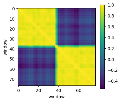
77 windows; mean FCD within halves 0.96, between halves -0.28

Summary

• A raster (np.nonzero on the spike matrix) and firing_rate describe activity; pass times as quantities so firing_rate returns Hz unambiguously.

• \(\kappa\) (cross_correlation) is not chance-corrected and grows with rate and bin width; compare with shuffled data.

• voltage_fluctuation returns Golomb’s \(\chi^2 \in [0, 1]\): about \(1/N\) for independent and 1 for identical traces.

• functional_connectivity is the correlation matrix of binned activity; the bin width selects the time scale. functional_connectivity_dynamics shows when that structure changes.