

Spike-Train Distances and Synchrony#
This tutorial covers the pairwise spike-train measures of braintools.analysis.spike. Each one answers a slightly different question, and several have properties that are easy to misread, so every section checks a function against a case with a known answer.
Function |
Input |
Measures |
|---|---|---|
|
spike times |
edit distance: shifting a spike by \(\Delta t\) costs \(q\lvert\Delta t\rvert\), adding or removing one costs 1 |
|
spike times |
distance between exponentially filtered trains |
|
spike matrix |
fraction of spikes with a partner in another train within the window |
|
spike matrix |
mean Pearson correlation of binned counts |
|
spike matrix |
STTC, a coincidence measure that is 0 for independent trains |
|
spike matrix |
locking of each neuron’s spikes to an external rhythm |
|
spike matrix |
co-occurrence of detected bursts |
The first two take arrays of spike times; the others take a (T, N) spike matrix plus dt. Pass time arguments as brainunit quantities and units are converted; the distance functions take plain numbers in one consistent unit.
1. Setup#
import brainunit as u
import jax.numpy as jnp
import matplotlib.pyplot as plt
import numpy as np

import braintools.analysis as ba

rng = np.random.default_rng(0)
dt = 1 * u.ms
2. Victor-Purpura Distance#
The distance is the cheapest way to turn one train into the other. The cost factor \(q\) (units of 1/time) sets the time scale: two spikes closer than \(2/q\) are cheaper to shift than to delete and re-insert. For \(q \to 0\) the distance is the difference in spike counts; for large \(q\) it counts the spikes that do not match exactly.
a = np.array([10.0, 30.0, 50.0, 70.0, 90.0])  # ms
b = a + 2.0  # every spike shifted by 2 ms
c = np.array([10.0, 50.0, 90.0])

print("identical:", ba.spike.victor_purpura_distance(a, a, cost_factor=1.0))
for q in [0.01, 0.1, 1.0, 10.0]:
    d = ba.spike.victor_purpura_distance(a, b, cost_factor=q)
    print(f"q = {q:5.2f}/ms: shifted by 2 ms -> {float(d):.2f}  (min(5 * q * 2, 10) = {min(5 * q * 2, 10):.2f})")
print("q -> 0, a vs c (5 vs 3 spikes):", float(ba.spike.victor_purpura_distance(a, c, cost_factor=1e-6)), "(count difference 2)")
identical: 0.0
q =  0.01/ms: shifted by 2 ms -> 0.10  (min(5 * q * 2, 10) = 0.10)
q =  0.10/ms: shifted by 2 ms -> 1.00  (min(5 * q * 2, 10) = 1.00)
q =  1.00/ms: shifted by 2 ms -> 10.00  (min(5 * q * 2, 10) = 10.00)
q = 10.00/ms: shifted by 2 ms -> 10.00  (min(5 * q * 2, 10) = 10.00)
q -> 0, a vs c (5 vs 3 spikes): 2.0 (count difference 2)
3. van Rossum Distance#
Each train is filtered with the causal kernel \(K(t) = \frac1\tau e^{-t/\tau}\) and the distance is \(D = \sqrt{\int (f_1 - f_2)^2\,dt}\). It is evaluated in closed form. For two single spikes a time \(\Delta\) apart,
so small shifts cost little when \(\tau \gg \Delta\), and \(D^2 \to 1/\tau\) (two unrelated spikes) when \(\Delta \gg \tau\).
print(f"{'tau':>5s} {'Delta':>6s} {'D':>8s} {'closed form':>12s}")
for tau in [1.0, 10.0]:
    for delta in [0.5, 5.0, 50.0]:
        D = float(ba.spike.van_rossum_distance(np.array([100.0]), np.array([100.0 + delta]), tau=tau, t_max=1000.0))
        print(f"{tau:5.0f} {delta:6.1f} {D:8.4f} {np.sqrt((1 - np.exp(-delta / tau)) / tau):12.4f}")
tau Delta D closed form
    1    0.5   0.6273       0.6273
    1    5.0   0.9966       0.9966
    1   50.0   1.0000       1.0000
   10    0.5   0.0698       0.0698
   10    5.0   0.1984       0.1984
   10   50.0   0.3152       0.3152
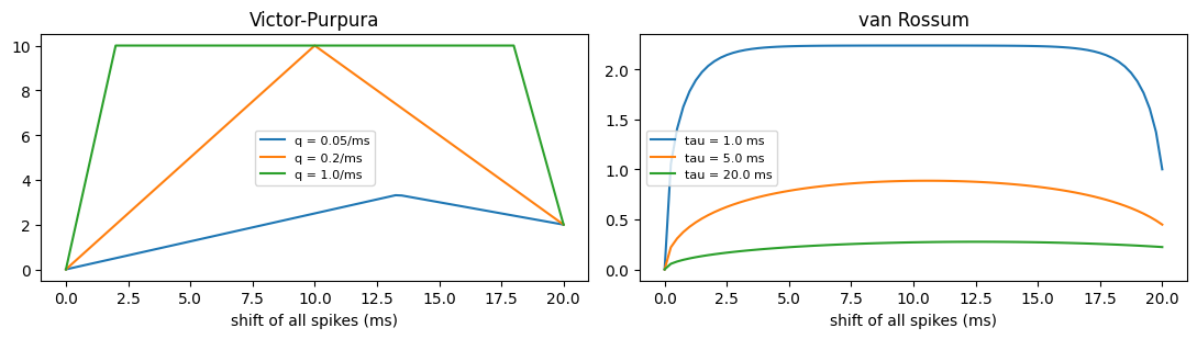
The default integration end is the last spike plus \(5\tau\), which leaves out less than \(e^{-10}\) of each kernel’s squared tail; pass t_max to integrate further. Here is the distance as a function of the shift between the two 5-spike trains:
shifts = np.linspace(0, 20, 81)
fig, axes = plt.subplots(1, 2, figsize=(11, 3.2))
for q in [0.05, 0.2, 1.0]:
    axes[0].plot(shifts, [float(ba.spike.victor_purpura_distance(a, a + s, cost_factor=q)) for s in shifts], label=f"q = {q}/ms")
for tau in [1.0, 5.0, 20.0]:
    axes[1].plot(shifts, [float(ba.spike.van_rossum_distance(a, a + s, tau=tau)) for s in shifts], label=f"tau = {tau} ms")
axes[0].set_title("Victor-Purpura")
axes[1].set_title("van Rossum")
for ax in axes:
    ax.set_xlabel("shift of all spikes (ms)")
    ax.legend(fontsize=8)
fig.tight_layout()
plt.show()
4. Coincidence Measures and Firing Rate#
Three functions summarize synchrony from a spike matrix:
spike_train_synchrony: for each pair, the fraction of spikes that have a partner in the other train withinwindow_size / 2, averaged over pairs. Between 0 and 1.correlation_index: the mean Pearson correlation of spike counts in bins ofwindow_size.spike_time_tiling_coefficient(STTC, Cutts & Eglen 2014): compares the fraction of A’s spikes within \(\pm\tau\) of a B spike with the fraction of time covered by \(\pm\tau\) windows around B’s spikes. Matrix output, 1 on the diagonal. The default is \(\tau = 5\) ms.
The crucial difference shows up with independent trains at increasing rates. A coincidence fraction grows simply because there are more spikes to coincide with, whereas STTC and the correlation index subtract what chance predicts:
T = 20_000  # 20 s at dt = 1 ms
print(f"{'rate':>6s} {'synchrony':>10s} {'corr. index':>12s} {'STTC':>7s}   independent trains, window 10 ms")
for rate in [2, 10, 50]:
    s = (rng.random((T, 10)) < rate * 1e-3).astype(float)
    sync = float(ba.spike.spike_train_synchrony(s, window_size=10 * u.ms, dt=dt))
    ci = float(ba.spike.correlation_index(s, window_size=10 * u.ms, dt=dt))
    sttc = np.asarray(ba.spike.spike_time_tiling_coefficient(s, dt=dt, tau=5 * u.ms))
    print(f"{rate:4d}Hz {sync:10.3f} {ci:12.3f} {sttc[np.triu_indices(10, 1)].mean():7.3f}")
rate synchrony corr. index STTC independent trains, window 10 ms
2Hz 0.023 0.001 0.001
10Hz 0.104 0.001 0.001
50Hz 0.435 0.005 0.004
With a real shared component the chance-corrected measures rise above zero. Ten trains share 100 events (each train joins 60 % of them, jittered by up to \(\pm 2\) ms) on top of 10 Hz background:
s = (rng.random((T, 10)) < 0.01).astype(float)
shared_events = rng.choice(np.arange(10, T - 10), 100, replace=False)
for e in shared_events:
    who = np.flatnonzero(rng.random(10) < 0.6)
    s[e + rng.integers(-2, 3, who.size), who] = 1
print(f"synchrony {float(ba.spike.spike_train_synchrony(s, window_size=10 * u.ms, dt=dt)):.3f}, "
      f"correlation index {float(ba.spike.correlation_index(s, window_size=10 * u.ms, dt=dt)):.3f}, "
      f"STTC {np.asarray(ba.spike.spike_time_tiling_coefficient(s, dt=dt))[np.triu_indices(10, 1)].mean():.3f}")
synchrony 0.258, correlation index 0.123, STTC 0.129
5. Phase Locking to a Rhythm#
phase_locking_value(spikes, reference_freq, dt) assigns each spike the phase \(\phi_k = 2\pi f t_k\) of a reference oscillation and returns the vector strength \(\lvert\frac1N\sum_k e^{i\phi_k}\rvert\) per neuron. If spikes occur at a preferred phase with Gaussian timing jitter \(\sigma_t\), the expected value is \(e^{-(2\pi f \sigma_t)^2/2}\).
f_ref = 20.0  # Hz
T = 200_000  # 200 s at 1 ms, 4000 cycles
jitters = [1.0, 3.0, 6.0, 10.0]  # ms
S = np.zeros((T, len(jitters)))
cycle_starts = np.arange(0, T, 1000 / f_ref)
for j, sd in enumerate(jitters):
    times = cycle_starts + 10.0 + rng.normal(0, sd, cycle_starts.size)  # preferred phase 10 ms into each cycle
    idx = np.clip(np.round(times).astype(int), 0, T - 1)
    S[idx, j] = 1

plv = np.asarray(ba.spike.phase_locking_value(S, f_ref, dt))
for sd, value in zip(jitters, plv):
    print(f"jitter {sd:4.1f} ms: PLV {value:.3f}, expected {np.exp(-(2 * np.pi * f_ref * sd * 1e-3) ** 2 / 2):.3f}")
jitter  1.0 ms: PLV 0.992, expected 0.992
jitter  3.0 ms: PLV 0.931, expected 0.931
jitter  6.0 ms: PLV 0.752, expected 0.753
jitter 10.0 ms: PLV 0.457, expected 0.454
reference_freq is in Hz; a plain-number dt here is in seconds (unlike the coincidence measures), which is another reason to pass a quantity. The PLV tests locking to an external rhythm; it says nothing about spike-to-spike synchrony.
6. Burst Synchrony#
burst_synchrony_index first detects bursts in each train (runs of at least burst_threshold spikes with inter-spike intervals up to max_isi), then returns the fraction of bursts that overlap in time with a burst of any other neuron. Like \(\kappa\), it is not chance-corrected: the more neurons and the more bursts, the more likely an overlap by accident. Compare aligned bursts with bursts at independent times, which give the chance level:
def bursting(aligned, n=8, T=10_000):
    s = np.zeros((T, n))
    shared = rng.choice(np.arange(100, T - 100), 15, replace=False)
    for i in range(n):
        starts = shared if aligned else rng.choice(np.arange(100, T - 100), 15, replace=False)
        for b in starts:
            s[b + np.arange(0, 25, 5) + rng.integers(0, 2, 5), i] = 1  # 5 spikes, 5 ms apart
    return s


for aligned in [True, False]:
    s = bursting(aligned)
    print(f"{'aligned' if aligned else 'independent'} bursts: index "
          f"{float(ba.spike.burst_synchrony_index(s, burst_threshold=3, max_isi=10 * u.ms, dt=dt)):.3f}")

# Chance level: two ~25 ms bursts overlap when their starts are within 25 ms (a 50 ms window
# out of 10 s); each burst has 7 x 15 = 105 bursts of other neurons it could overlap.
print(f"chance level for independent timing: {1 - (1 - 50 / 10_000) ** 105:.2f}")
aligned bursts: index 1.000
independent bursts: index 0.409
chance level for independent timing: 0.41
Summary#
Victor-Purpura and van Rossum distances compare two trains; their parameter (\(q\) or \(\tau\)) sets the temporal precision that counts as “the same”.
Raw coincidence fractions (
spike_train_synchrony) grow with firing rate even for independent trains. STTC and the correlation index stay near 0 for independent trains.phase_locking_valuemeasures locking to an external frequency; with Gaussian jitter it matches \(e^{-(2\pi f\sigma_t)^2/2}\).burst_synchrony_indexcompares burst timing across neurons; like \(\kappa\) it has a chance level that grows with the number of neurons and bursts.Pass times as quantities: plain numbers mean milliseconds for the coincidence and burst measures but seconds for
phase_locking_value.