The analysis toolbox: spikes, spectra and populations

This tutorial walks through the measures added to braintools.analysis in 0.4. Each section builds data with a known answer and checks the measure against it:

1. Spike-train statistics on a SpikeTrains: ISI, CV, CV2, LV, Fano factor, PSTH, correlograms, spike-triggered averages and spike-train distances.

2. Spectral analysis of continuous signals: multitaper spectra, Morlet wavelets, band-pass filtering and phase synchrony.

3. Population analysis: PCA, decoding, Granger causality and neuronal avalanches.

4. Resampling: significance tests with jittered spikes and phase-randomised signals, and bootstrap confidence intervals.

Every function here runs under jax.jit and jax.vmap and accepts brainunit quantities.

import brainunit as u
import jax
import jax.numpy as jnp
import matplotlib.pyplot as plt
import numpy as np

from braintools.analysis import population, spectral, spike, stats
from braintools.spike import SpikeTrains

1. Spike-train statistics

We simulate two populations for 20 s at 0.1 ms resolution: 20 Poisson neurons (irregular, CV ≈ 1) and 20 regular neurons that fire every 50 ms with a little jitter (CV ≈ 0). A dense raster becomes a SpikeTrains with SpikeTrains.from_dense; its capacity is the largest spike count of any neuron.

dt = 0.1 * u.ms
n_steps = 200_000  # 20 s
rng = np.random.default_rng(0)

poisson = rng.random((n_steps, 20)) < 20.0 * 1e-4          # 20 Hz
regular = np.zeros((n_steps, 20), dtype=bool)
period = 500                                                 # 50 ms in steps
for i in range(20):  # building the toy data on the host is fine
    t = np.arange(rng.integers(0, period), n_steps, period)
    t = np.clip(t + rng.integers(-5, 6, size=t.size), 0, n_steps - 1)
    regular[t, i] = True

trains = SpikeTrains.from_dense(np.concatenate([poisson, regular], axis=1), dt=dt)
trains

SpikeTrains(n_neurons=40, capacity=436, n_spikes=15892, t_start=0. ms, t_stop=20000. ms, overflow=False)

cv, cv2, lv = spike.cv(trains), spike.cv2(trains), spike.lv(trains)
print('CV   Poisson %.2f  regular %.2f' % (cv[:20].mean(), cv[20:].mean()))
print('CV2  Poisson %.2f  regular %.2f' % (cv2[:20].mean(), cv2[20:].mean()))
print('LV   Poisson %.2f  regular %.2f' % (lv[:20].mean(), lv[20:].mean()))
ff = spike.fano_factor(trains, bin_size=100 * u.ms)
print('Fano factor (100 ms bins)  Poisson %.2f  regular %.2f' % (ff[:20].mean(), ff[20:].mean()))

CV   Poisson 0.99  regular 0.01
CV2  Poisson 1.00  regular 0.01
LV   Poisson 0.99  regular 0.00

Fano factor (100 ms bins)  Poisson 0.98  regular 0.00

For a Poisson process CV, CV2, LV and the Fano factor are all close to 1; for the regular population they are close to 0. Undefined values (a neuron with fewer than two intervals) come back as nan rather than raising, so the statistics work inside jit.

PSTH and spike-triggered average

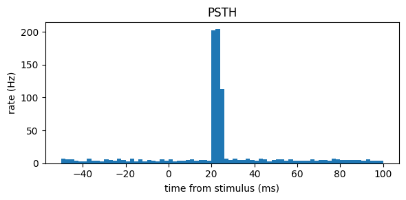
psth aligns spikes to event times. Here a population responds 20 ms after each of 50 stimuli; the PSTH recovers the response latency.

events = np.arange(50) * 0.4 + 0.2            # stimulus times in s
resp = rng.random((n_steps, 30)) < 5e-4         # 5 Hz background
for e in events:
    k = int(round((e + 0.020) / 1e-4))
    resp[k:k + 50] |= rng.random((50, 30)) < 0.02  # 5 ms burst, 20 ms after the event
resp_trains = SpikeTrains.from_dense(resp, dt=dt)

rate, edges = spike.psth(resp_trains, events * u.second, window=(50 * u.ms, 100 * u.ms), bin_size=2 * u.ms)
centers = (edges[:-1] + edges[1:]) / 2
plt.figure(figsize=(6, 3))
plt.bar(centers.to_decimal(u.ms), rate.mean(axis=1), width=2)
plt.xlabel('time from stimulus (ms)'); plt.ylabel('rate (Hz)'); plt.title('PSTH')
plt.tight_layout()
print('peak at %.0f ms' % centers.to_decimal(u.ms)[int(jnp.argmax(rate.mean(axis=1)))])

peak at 23 ms

Correlograms

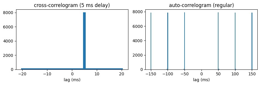
cross_correlogram compares neuron i of one SpikeTrains with neuron i of another. A copy of the Poisson trains delayed by 5 ms produces a peak at +5 ms; the auto-correlogram of the regular neurons shows their 50 ms period.

delayed = np.roll(poisson, 50, axis=0)           # 5 ms later
a = SpikeTrains.from_dense(poisson, dt=dt)
b = SpikeTrains.from_dense(delayed, dt=dt)
ccg, lags = spike.cross_correlogram(a, b, bin_size=1 * u.ms, max_lag=20 * u.ms)
acg, alags = spike.auto_correlogram(trains.select(np.arange(20, 40)), bin_size=2 * u.ms, max_lag=150 * u.ms)

fig, axes = plt.subplots(1, 2, figsize=(9, 3))
axes[0].bar(lags.to_decimal(u.ms), ccg.sum(axis=0), width=1)
axes[0].set(xlabel='lag (ms)', title='cross-correlogram (5 ms delay)')
axes[1].bar(alags.to_decimal(u.ms), acg.sum(axis=0), width=2)
axes[1].set(xlabel='lag (ms)', title='auto-correlogram (regular)')
plt.tight_layout()

Spike-train distances

The ISI- and SPIKE-distances of Kreuz et al. are 0 for identical trains and grow as the trains diverge. Both compare neuron i of one SpikeTrains with neuron i of another and vectorise over neurons; jittering spikes by increasing amounts makes the distances grow.

key = jax.random.key(1)
widths = [0.5, 2.0, 8.0, 32.0]
for w in widths:
    jittered = stats.jitter_spikes(key, a, w * u.ms)
    print('jitter %5.1f ms   ISI-distance %.3f   SPIKE-distance %.3f'
          % (w, spike.isi_distance(a, jittered).mean(), spike.spike_distance(a, jittered).mean()))

jitter   0.5 ms   ISI-distance 0.009   SPIKE-distance 0.005
jitter   2.0 ms   ISI-distance 0.034   SPIKE-distance 0.018
jitter   8.0 ms   ISI-distance 0.112   SPIKE-distance 0.064

jitter  32.0 ms   ISI-distance 0.277   SPIKE-distance 0.176

2. Spectral analysis

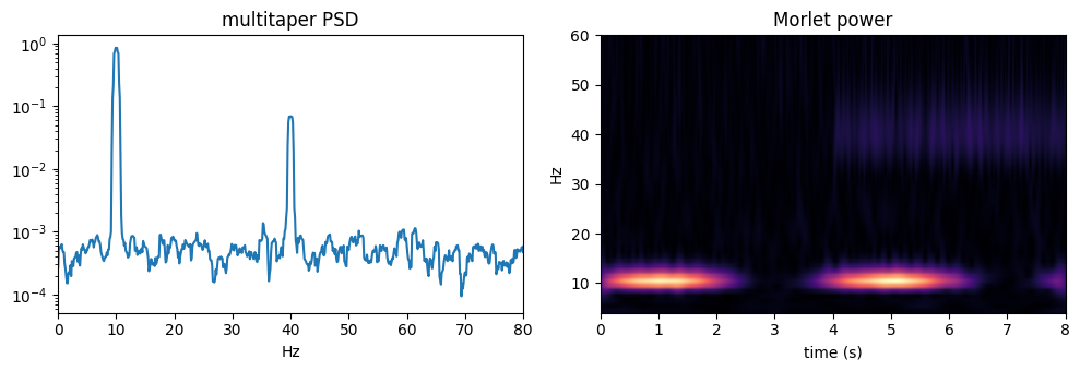
A 10 Hz rhythm whose amplitude is modulated, plus a 40 Hz component and noise, sampled at 1 kHz. The multitaper estimate has much lower variance than a single periodogram; the Morlet transform shows when each rhythm is present.

fs = 1000.0
t = np.arange(0, 8, 1 / fs)
alpha = (1 + np.sin(2 * np.pi * 0.25 * t)) * np.sin(2 * np.pi * 10 * t)
gamma = 0.5 * np.sin(2 * np.pi * 40 * t) * (t > 4)
x = jnp.asarray(alpha + gamma + 0.5 * rng.standard_normal(t.size))

freqs, psd = spectral.multitaper_psd(x, dt=1 * u.ms, nw=4.0)
wfreqs = jnp.arange(4.0, 60.0, 1.0)
tfr = spectral.morlet_transform(x, dt=1 * u.ms, freqs=wfreqs, n_cycles=7.0)

fig, axes = plt.subplots(1, 2, figsize=(10, 3.5))
axes[0].semilogy(freqs, psd); axes[0].set(xlim=(0, 80), xlabel='Hz', title='multitaper PSD')
axes[1].imshow(jnp.abs(tfr), aspect='auto', origin='lower', extent=(0, 8, 4, 60), cmap='magma')
axes[1].set(xlabel='time (s)', ylabel='Hz', title='Morlet power')
plt.tight_layout()
print('alpha band power fraction %.2f' % spectral.band_power(x, dt=1 * u.ms, band=(8, 12), nperseg=1000, relative=True))

alpha band power fraction 0.72

Band-pass filtering and phase synchrony

bandpass is a zero-phase Butterworth filter (it matches scipy.signal.sosfiltfilt) that runs inside jit. Two noisy signals sharing a 10 Hz rhythm with a fixed lag are phase-locked in the alpha band but not in an unrelated band: plv is high and wpli (insensitive to zero-lag volume conduction) is also high because the lag is non-zero.

y = jnp.asarray(np.sin(2 * np.pi * 10 * t - 0.8) + 0.8 * rng.standard_normal(t.size))
z = jnp.asarray(np.sin(2 * np.pi * 10 * t) + 0.8 * rng.standard_normal(t.size))
for band in [(8, 12), (25, 35)]:
    print('band %-8s PLV %.2f   PLI %.2f   wPLI %.2f' % (
        band, spectral.plv(y, z, dt=1 * u.ms, band=band),
        spectral.pli(y, z, dt=1 * u.ms, band=band), spectral.wpli(y, z, dt=1 * u.ms, band=band)))

band (8, 12)  PLV 0.99   PLI 0.99   wPLI 1.00

band (25, 35) PLV 0.05   PLI 0.02   wPLI 0.13

3. Population analysis

Low-dimensional structure and decoding

100 neurons are driven by a 3-dimensional latent signal whose variances are in the ratio 9 : 4 : 1. PCA finds that three components explain almost all the variance. The participation ratio \((\sum\lambda)^2/\sum\lambda^2\) is an effective dimensionality that weights each dimension by its variance, so it comes out near \(14^2/98 = 2\) rather than 3. decode then predicts which of four stimuli was shown from noisy population responses, with cross-validation.

latent = rng.standard_normal((2000, 3)) * np.array([3.0, 2.0, 1.0])
mixing = rng.standard_normal((3, 100))
activity = jnp.asarray(latent @ mixing + 0.3 * rng.standard_normal((2000, 100)))
res = population.pca(activity, n_components=10)
print('explained variance ratio of the first 4 PCs:', np.round(res.explained_variance_ratio[:4], 3))
print('participation ratio: %.2f' % population.participation_ratio(activity))

labels = jnp.asarray(rng.integers(0, 4, size=400))
templates = rng.standard_normal((4, 50))
responses = jnp.asarray(templates[np.asarray(labels)] + 2.0 * rng.standard_normal((400, 50)))
acc = population.decode(responses, labels, n_folds=5, model='lda', reg=0.1, key=jax.random.key(0))
print('decoding accuracy per fold:', np.round(acc, 2), '(chance 0.25)')

explained variance ratio of the first 4 PCs: [0.669 0.259 0.067 0.   ]
participation ratio: 1.93

decoding accuracy per fold: [1.         0.94       0.97999996 0.98999995 0.96      ] (chance 0.25)

Granger causality and avalanches

In a three-node chain x → y → z, conditional Granger causality finds the two direct links and no direct x → z link. avalanches splits a population count series into bursts separated by silence; for a critical branching process the branching ratio is close to 1.

T = 5000
xyz = np.zeros((T, 3))
noise = rng.standard_normal((T, 3))
for k in range(1, T):  # toy data generation on the host
    xyz[k, 0] = 0.5 * xyz[k - 1, 0] + noise[k, 0]
    xyz[k, 1] = 0.5 * xyz[k - 1, 1] + 0.8 * xyz[k - 1, 0] + noise[k, 1]
    xyz[k, 2] = 0.5 * xyz[k - 1, 2] + 0.8 * xyz[k - 1, 1] + noise[k, 2]
gc = population.granger_causality(jnp.asarray(xyz), order=2)
print('GC[target, source]:')
print(np.round(gc, 3))

# a branching process with ratio sigma, restarted by rare external input
sigma, counts = 1.0, np.zeros(20000, dtype=int)
for k in range(1, counts.size):
    counts[k] = rng.poisson(sigma * counts[k - 1]) + (rng.random() < 0.01)
av = population.avalanches(jnp.asarray(counts))
print('avalanches:', int(av.n), ' branching ratio: %.2f' % population.branching_ratio(jnp.asarray(counts)))

GC[target, source]:
[[0.         0.         0.001     ]
 [0.55200005 0.         0.001     ]
 [0.001      0.60800004 0.        ]]

avalanches: 181  branching ratio: 0.99

4. Resampling and confidence intervals

Is the 5 ms delayed coupling from section 1 significant? Compare the observed coincidence count with a null distribution built by jittering one train; jax.lax.map over the keys (vectorised in batches of 10) builds the whole null distribution in one compiled call. For continuous signals, phase_randomize keeps the power spectrum but destroys phase relations between signals. (It needs a broadband or noisy signal: a pure sinusoid is a single Fourier component, which phase randomisation merely shifts.) Finally, bootstrap_ci gives a confidence interval for any statistic.

def coincidences(b_trains):
    ccg, _ = spike.cross_correlogram(a, b_trains, bin_size=1 * u.ms, max_lag=20 * u.ms)
    return ccg[:, 25].sum()  # the +5 ms bin

observed = coincidences(b)
keys = jax.random.split(jax.random.key(2), 200)
# lax.map with batch_size vmaps 10 keys at a time, bounding memory
null = jax.lax.map(lambda k: coincidences(stats.jitter_spikes(k, b, 10 * u.ms)), keys, batch_size=10)
print('observed %d, null mean %.1f, p = %.3f' % (observed, null.mean(), (null >= observed).mean()))

# two signals sharing a narrow-band (8-12 Hz) noise driver with a 20 ms lag
drive = np.asarray(spectral.bandpass(jnp.asarray(rng.standard_normal(t.size + 20)), dt=1 * u.ms, band=(8, 12)))
p = jnp.asarray(drive[20:] + 0.02 * rng.standard_normal(t.size))
q = jnp.asarray(drive[:-20] + 0.02 * rng.standard_normal(t.size))
surr = stats.phase_randomize(jax.random.key(3), p)
print('PLV original %.2f, phase-randomised %.2f' % (
    spectral.plv(p, q, dt=1 * u.ms, band=(8, 12)), spectral.plv(surr, q, dt=1 * u.ms, band=(8, 12))))

low, high = stats.bootstrap_ci(jax.random.key(4), cv[:20], jnp.nanmean, n_resamples=2000)
print('mean CV of the Poisson neurons: 95%% CI [%.3f, %.3f]' % (low, high))

observed 8019, null mean 545.9, p = 0.000

PLV original 0.96, phase-randomised 0.22

mean CV of the Poisson neurons: 95% CI [0.969, 1.012]

Summary

Task	Functions
interval statistics	spike.isi, cv, cv2, lv, fano_factor
event-aligned	spike.psth, spike_triggered_average
pairwise timing	spike.cross_correlogram, auto_correlogram, isi_distance, spike_distance
spectra	spectral.multitaper_psd, spectrogram, morlet_transform, band_power
filtering and phase	spectral.bandpass, analytic_signal, plv, pli, wpli
population	population.pca, participation_ratio, cca, rdm, rsa, decode, mutual_information
collective dynamics	population.kuramoto_order_parameter, granger_causality, avalanches, branching_ratio
resampling	stats.jitter_spikes, shuffle_isi, phase_randomize, bootstrap_ci

See the API reference for every parameter.