Readout learning, regression and multi-start search

Besides gradient-based optimizers, braintools.optim has tools for problems with more structure:

1. FORCE learning (FORCE): train the linear readout of a chaotic recurrent rate network online, so that the network produces a target signal on its own.

2. Online least squares (RLS, LMS) against the closed-form ridge_regression on the same linear problem.

3. Sparse regression (lasso_regression, elastic_net_regression): how the number of selected features shrinks as the penalty alpha grows.

4. Multi-start minimization (multistart_minimize): a local optimizer run from hundreds of starting points at once on a multimodal function.

Every repeated model step below runs inside brainstate.transform.for_loop, which compiles the whole time loop into one XLA program.

import brainstate
import jax
import jax.numpy as jnp
import matplotlib.pyplot as plt
import numpy as np

import braintools
from braintools.optim import (
    FORCE, LMS, RLS,
    elastic_net_regression, lasso_regression, ridge_regression,
    multistart_init, multistart_minimize,
)

1. FORCE learning on a chaotic rate network

The network has \(N\) rate units with state \(x\), rates \(r = \tanh(x)\) and a linear readout \(z = w^\top r\) that is fed back into every unit:

\[\tau \dot x = -x + J r + w_{fb}\, z .\]

The recurrent weights \(J_{ij} \sim \mathcal N(0, g^2/N)\) with gain \(g = 1.5 > 1\) make the network chaotic when the readout is silent. FORCE learning (Sussillo and Abbott, 2009) trains only \(w\), by recursive least squares at every time step, so that \(z\) follows a target \(f(t)\). Because the RLS update is strong from the first step, the error stays small throughout, the fed-back signal is close to the target, and the network’s chaos is tamed into the periodic activity that generates \(f\).

The target here is a sum of three sines with periods of 240, 120 and 60 ms. The state lives in brainstate states: x is a HiddenState, the readout w a ParamState registered with the optimizer.

N, g, dt, tau = 400, 1.5, 1.0, 10.0          # time in ms
k_J, k_fb, k_x = jax.random.split(jax.random.PRNGKey(0), 3)
J = g * jax.random.normal(k_J, (N, N)) / jnp.sqrt(N)
w_fb = jax.random.uniform(k_fb, (N,), minval=-1.0, maxval=1.0)

x = brainstate.HiddenState(0.5 * jax.random.normal(k_x, (N,)))
w = brainstate.ParamState(jnp.zeros((N, 1)))
force = FORCE(alpha=1.0)
force.register_trainable_weights({'readout': w})


def target_fn(t):
    return (jnp.sin(2 * jnp.pi * t / 240.) + 0.5 * jnp.sin(2 * jnp.pi * t / 120.)
            + 0.25 * jnp.sin(2 * jnp.pi * t / 60.)) / 1.5


def step(target, train):
    # One Euler step of the network; with train=True, one FORCE update of the readout.
    r = jnp.tanh(x.value)
    z = r @ w.value                                  # readout, shape (1,)
    x.value = x.value + dt / tau * (-x.value + J @ r + w_fb * z[0])
    if train:
        w_old = w.value
        force.step(r[None], z[None], target[None])   # inputs, current output, target
        dw = jnp.linalg.norm(w.value - w_old)
    else:
        dw = jnp.zeros(())
    return z[0], r[:5], dw

The run has three phases, each a single for_loop over the target samples: 1 s of spontaneous activity (the readout is still zero, so there is no feedback), 6 s of training, and 2 s of testing with learning switched off, where the network runs on its own feedback.

T_pre, T_train, T_test = 1000, 6000, 2000
t = jnp.arange(T_pre + T_train + T_test) * dt
f = target_fn(t)[:, None]
f_pre, f_train, f_test = f[:T_pre], f[T_pre:T_pre + T_train], f[T_pre + T_train:]

z_pre, r_pre, _ = brainstate.transform.for_loop(lambda y: step(y, False), f_pre)
z_train, r_train, dw_train = brainstate.transform.for_loop(lambda y: step(y, True), f_train)
z_test, r_test, _ = brainstate.transform.for_loop(lambda y: step(y, False), f_test)

def mse(z, y):
    return float(jnp.mean((z - y[:, 0]) ** 2))

print('target variance:            %.4f' % float(jnp.var(f)))
print('training MSE, first 500 ms: %.2e' % mse(z_train[:500], f_train[:500]))
print('training MSE, last 500 ms:  %.2e' % mse(z_train[-500:], f_train[-500:]))
print('test MSE (no learning):     %.2e' % mse(z_test, f_test))

target variance:            0.2916
training MSE, first 500 ms: 1.43e-03
training MSE, last 500 ms:  7.02e-06

test MSE (no learning):     1.19e-04

segments = [('before: spontaneous', t[:T_pre], r_pre, z_pre, f_pre),
            ('during: first 1 s of training', t[T_pre:T_pre + 1000], r_train[:1000], z_train[:1000], f_train[:1000]),
            ('after: learning off', t[T_pre + T_train:], r_test, z_test, f_test)]
fig, axes = plt.subplots(2, 3, figsize=(12, 5), sharey='row')
for col, (title, ts, rates, z, y) in enumerate(segments):
    axes[0, col].plot(ts, rates, lw=0.8)
    axes[0, col].set_title(title)
    axes[1, col].plot(ts, y[:, 0], 'k--', lw=1.2, label='target')
    axes[1, col].plot(ts, z, color='tab:red', lw=1, label='readout z')
    axes[1, col].set_xlabel('time (ms)')
axes[0, 0].set_ylabel('rates of 5 units')
axes[1, 0].set_ylabel('output')
axes[1, 0].legend(loc='lower left', fontsize=8)
plt.tight_layout()

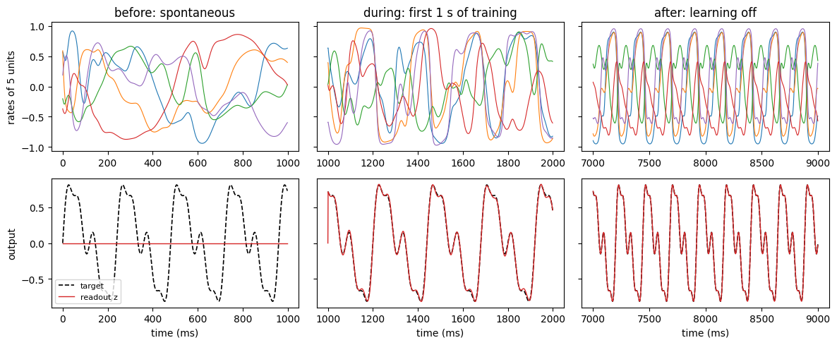
Before training the readout is zero and the units fluctuate irregularly: this is the chaotic regime of \(g = 1.5\). Within a few steps of training the readout follows the target closely (a training MSE of 1.4e-3 over the first 500 ms, against a target variance of 0.29), and the unit activity becomes periodic, locked to the 240 ms period of the target. By the end of training the error has fallen to 7.0e-6. With learning switched off, the network keeps generating the target from its own feedback, with a test MSE of 1.2e-4.

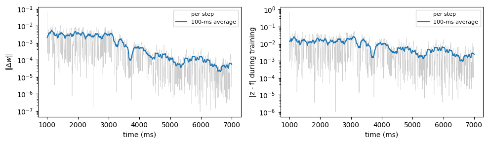
The size of each readout update, \(\|\Delta w\|\), shows the learning settling down, while the error stays small throughout, so FORCE never has to correct large deviations:

err_train = np.abs(np.asarray(z_train) - np.asarray(f_train[:, 0]))
dw = np.asarray(dw_train)
window = np.ones(100) / 100                       # 100-ms moving average
t_ms = np.asarray(t[T_pre:T_pre + T_train])
fig, axes = plt.subplots(1, 2, figsize=(10, 3))
axes[0].semilogy(t_ms, dw, color='0.8', lw=0.4, label='per step')
axes[0].semilogy(t_ms, np.convolve(dw, window, mode='same'), lw=1.5, label='100-ms average')
axes[0].set_xlabel('time (ms)'); axes[0].set_ylabel(r'$\|\Delta w\|$'); axes[0].legend(fontsize=8)
axes[1].semilogy(t_ms, err_train, color='0.8', lw=0.4, label='per step')
axes[1].semilogy(t_ms, np.convolve(err_train, window, mode='same'), lw=1.5, label='100-ms average')
axes[1].set_xlabel('time (ms)'); axes[1].set_ylabel('|z - f| during training'); axes[1].legend(fontsize=8)
plt.tight_layout()
print('mean |dw| over the first / last 100 steps: %.1e / %.1e'
      % (float(dw_train[:100].mean()), float(dw_train[-100:].mean())))

mean |dw| over the first / last 100 steps: 3.6e-03 / 6.3e-05

2. Online least squares: RLS, LMS and ridge_regression

FORCE is RLS applied inside a recurrent network. On a plain linear problem \(y = X w + \varepsilon\), RLS with forgetting factor 1 does something exact: after any number of samples its weights equal the ridge solution

\[\arg\min_W \|Y - X W\|^2 + \alpha \|W\|^2\]

over the samples seen so far (with zero initial weights and \(P_0 = I/\alpha\)). Here 400 noisy samples with 20 features are fed to RLS one at a time inside a for_loop, recording the weights after every sample:

rng = np.random.default_rng(0)
n, d, alpha = 400, 20, 5.0
X = rng.normal(size=(n, d)).astype(np.float32)
w_true = rng.normal(size=(d, 1)).astype(np.float32)
Y = X @ w_true + 0.5 * rng.normal(size=(n, 1)).astype(np.float32)

w_rls = brainstate.ParamState(jnp.zeros((d, 1)))
rls = RLS(alpha=alpha)
rls.register_trainable_weights({'w': w_rls})

def rls_step(x_i, y_i):
    rls.step(x_i[None], None, y_i[None])     # outputs=None: computed as x @ w
    return w_rls.value[:, 0]

w_history = brainstate.transform.for_loop(rls_step, jnp.asarray(X), jnp.asarray(Y))

ridge_all = ridge_regression(X, Y, alpha=alpha, fit_intercept=False)
ridge_50 = ridge_regression(X[:50], Y[:50], alpha=alpha, fit_intercept=False)
print('max |RLS - ridge|, all 400 samples:   %.1e' % float(jnp.max(jnp.abs(w_rls.value - ridge_all.coef))))
print('max |RLS - ridge|, first 50 samples:  %.1e' % float(jnp.max(jnp.abs(w_history[49] - ridge_50.coef[:, 0]))))

max |RLS - ridge|, all 400 samples:   1.8e-06
max |RLS - ridge|, first 50 samples:  8.9e-07

The two agree to float32 rounding (about 1e-6), after all 400 samples and after the first 50 alike: RLS needs no learning rate, and after every sample it holds the best regularised fit to the data seen so far. The price is the \(d \times d\) matrix \(P\) that it updates at every step.

LMS (Widrow-Hoff) is the first-order counterpart: \(w \leftarrow w - \eta\, x\, e\) per sample, with no \(P\) matrix. It is cheaper per step but needs a learning rate, and it is stable only for \(\eta < 2/\|x\|^2\), about \(2/d = 0.1\) here. Each run below is one for_loop over the same samples:

def run_lms(lr):
    w_lms = brainstate.ParamState(jnp.zeros((d, 1)))
    lms = LMS(lr=lr)
    lms.register_trainable_weights({'w': w_lms})

    def lms_step(x_i, y_i):
        lms.step(x_i[None], None, y_i[None])
        return jnp.linalg.norm(w_lms.value[:, 0] - w_true[:, 0])

    return np.asarray(brainstate.transform.for_loop(lms_step, jnp.asarray(X), jnp.asarray(Y)))


lms_rates = [0.002, 0.01, 0.05, 0.12]
lms_errors = {lr: run_lms(lr) for lr in lms_rates}
rls_error = np.asarray(jnp.linalg.norm(w_history - w_true[:, 0], axis=1))
ridge_error = float(jnp.linalg.norm(ridge_all.coef - w_true))

print('|w - w_true| after 400 samples:')
print('  ridge (closed form): %.3f' % ridge_error)
print('  RLS:                 %.3f' % rls_error[-1])
for lr in lms_rates:
    print('  LMS lr=%-5g          %.3g' % (lr, lms_errors[lr][-1]))

fig, ax = plt.subplots(figsize=(6.5, 3.5))
samples = np.arange(1, n + 1)
ax.semilogy(samples, rls_error, 'k', lw=2, label='RLS')
for lr in lms_rates:
    ax.semilogy(samples, lms_errors[lr], lw=1, label=f'LMS lr={lr}')
ax.axhline(ridge_error, color='k', ls=':', label='ridge (all samples)')
ax.set_ylim(0.05, 50); ax.set_xlabel('samples seen'); ax.set_ylabel(r'$\|w - w_{true}\|$')
ax.legend(fontsize=8, ncol=2); plt.tight_layout()

|w - w_true| after 400 samples:
  ridge (closed form): 0.094
  RLS:                 0.094
  LMS lr=0.002          1.89
  LMS lr=0.01           0.238
  LMS lr=0.05           0.66
  LMS lr=0.12           1.54e+05

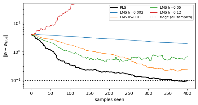
RLS ends at the ridge solution, 0.094 away from the true weights; that remaining error comes from the measurement noise and cannot be removed. The LMS runs show the learning-rate trade-off. With lr=0.002 LMS is still far off after 400 samples (1.89). lr=0.05 descends fastest at first but then stalls at a noise floor (0.66 at the end), because with a constant learning rate every noisy sample keeps pushing the weights around. lr=0.01 is the best of these rates (0.238). lr=0.12 is above the stability limit and diverges (1.5e5).

3. Sparse regression: lasso and elastic net

When only a few of many features matter, an \(L_1\) penalty sets the other coefficients exactly to zero. lasso_regression minimises the objective of scikit-learn’s Lasso,

\[\frac{1}{2n}\|y - X w - b\|^2 + \alpha \|w\|_1 ,\]

and elastic_net_regression adds an \(L_2\) term, \(\alpha\left(\rho \|w\|_1 + \tfrac{1-\rho}{2}\|w\|^2\right)\) with \(\rho\) = l1_ratio. Both are solved by FISTA inside a lax.while_loop, so they can be jax.vmap-ped over alpha to compute a whole regularisation path in one call.

The problem has 80 samples and 40 features, of which only the first 5 have non-zero true coefficients:

rng = np.random.default_rng(1)
n2, d2 = 80, 40
X2 = rng.normal(size=(n2, d2)).astype(np.float32)
coef_true = np.zeros(d2, np.float32)
coef_true[:5] = [3.0, -2.0, 1.5, -1.0, 0.5]
y2 = X2 @ coef_true + 0.3 * rng.normal(size=n2).astype(np.float32)

alphas = jnp.logspace(-3, 0.5, 30)
lasso_path = jax.vmap(lambda a: lasso_regression(X2, y2, alpha=a).coef)(alphas)
enet_path = jax.vmap(lambda a: elastic_net_regression(X2, y2, alpha=a, l1_ratio=0.5).coef)(alphas)

nnz_lasso = np.asarray((jnp.abs(lasso_path) > 0).sum(axis=1))
nnz_enet = np.asarray((jnp.abs(enet_path) > 0).sum(axis=1))
for i in [0, 10, 15, 20, 25, 29]:
    print('alpha = %7.4f   non-zero coefficients: lasso %2d, elastic net %2d'
          % (float(alphas[i]), nnz_lasso[i], nnz_enet[i]))

fit = lasso_regression(X2, y2, alpha=0.1)
print('\nlasso, alpha=0.1: first 8 coefficients', np.round(np.asarray(fit.coef[:8]), 3))
print('                  non-zero:', int((fit.coef != 0).sum()), ' true:', coef_true[:8])

true_support = coef_true != 0
exact = np.all((np.asarray(lasso_path) != 0) == true_support, axis=1)
print('\nalphas where the lasso support is exactly the true one: %.3f to %.3f (%d of 30 grid values)'
      % (float(alphas[exact].min()), float(alphas[exact].max()), exact.sum()))
print('elastic net, fewest non-zero coefficients below alpha = 1:', nnz_enet[np.asarray(alphas) < 1].min())

alpha =  0.0010   non-zero coefficients: lasso 40, elastic net 40
alpha =  0.0161   non-zero coefficients: lasso 22, elastic net 32
alpha =  0.0646   non-zero coefficients: lasso  8, elastic net 17
alpha =  0.2593   non-zero coefficients: lasso  5, elastic net  7
alpha =  1.0405   non-zero coefficients: lasso  3, elastic net  6
alpha =  3.1623   non-zero coefficients: lasso  0, elastic net  1

lasso, alpha=0.1: first 8 coefficients [ 2.851 -1.887  1.347 -0.942  0.395  0.    -0.     0.   ]
                  non-zero: 5  true: [ 3.  -2.   1.5 -1.   0.5  0.   0.   0. ]

alphas where the lasso support is exactly the true one: 0.113 to 0.452 (6 of 30 grid values)
elastic net, fewest non-zero coefficients below alpha = 1: 6

fig, axes = plt.subplots(1, 3, figsize=(13, 3.6))
a = np.asarray(alphas)
for ax, path, title in [(axes[0], lasso_path, 'lasso'), (axes[1], enet_path, 'elastic net (l1_ratio=0.5)')]:
    path = np.asarray(path)
    ax.semilogx(a, path[:, 5:], color='0.75', lw=0.8)
    for j in range(5):
        ax.semilogx(a, path[:, j], lw=2, label=f'w{j} (true {coef_true[j]:g})')
    ax.axhline(0, color='k', lw=0.5)
    ax.set_xlabel('alpha'); ax.set_ylabel('coefficient'); ax.set_title(title)
axes[0].legend(fontsize=7)
axes[2].semilogx(a, nnz_lasso, 'o-', ms=3, label='lasso')
axes[2].semilogx(a, nnz_enet, 's-', ms=3, label='elastic net')
axes[2].axhline(5, color='k', ls=':', label='true support (5)')
axes[2].set_xlabel('alpha'); axes[2].set_ylabel('non-zero coefficients'); axes[2].legend(fontsize=8)
plt.tight_layout()

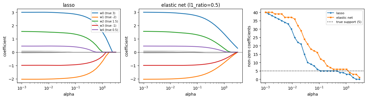
At the smallest alpha every coefficient is non-zero (40 of 40): with 80 samples for 40 features, the fit also follows the noise. As alpha grows the irrelevant coefficients drop out first, and between alpha = 0.113 and 0.452 the lasso selects exactly the 5 true features. Their estimates are shrunk towards zero: at alpha=0.1, for example, 2.851 for a true 3. Larger penalties then remove true features too, the smallest one (w4, true value 0.5) first. The elastic net keeps at least as many coefficients at every alpha (its \(L_1\) part is only half as strong, and its \(L_2\) part shrinks coefficients without setting them to zero); below alpha = 1 it never gets under 6 non-zero coefficients, so in that range it never isolates the true support.

4. Multi-start minimization of a multimodal function

The 2-D Rastrigin function

\[f(p) = 20 + \sum_{i=1}^{2} \left(p_i^2 - 10 \cos 2\pi p_i\right), \qquad p \in [-5.12, 5.12]^2,\]

has a local minimum near every integer point of the grid and its global minimum \(f = 0\) at the origin. A local optimizer finds the minimum of whichever basin it lands in, so it is run from many starts: multistart_init draws them uniformly in the box, and multistart_minimize runs L-BFGS from all of them at once (a vmap over a lax.while_loop, compiled into one program). With bounds, every start is optimised in an unconstrained space through a sigmoid, so the iterates never leave the box.

def rastrigin(p):
    return 20.0 + jnp.sum(p ** 2 - 10.0 * jnp.cos(2 * jnp.pi * p))


box = (jnp.full(2, -5.12), jnp.full(2, 5.12))
x0 = multistart_init(jax.random.PRNGKey(0), box, n_starts=512)
res = multistart_minimize(rastrigin, x0, method='lbfgs', bounds=(-5.12, 5.12), max_iter=100)

fun = np.asarray(res.fun)
print('starts:', x0.shape[0], ' converged:', int(res.converged.sum()),
      ' iterations: median %d, max %d' % (np.median(res.n_iter), int(res.n_iter.max())))
print('best start: #%d, f = %.2e at p = %s' % (int(res.best_index), float(res.best_fun), np.round(np.asarray(res.best_x), 4)))
print('it started at', np.round(np.asarray(x0[res.best_index]), 3))
print('starts reaching f < 1e-3:', int((fun < 1e-3).sum()))
levels, counts = np.unique(np.round(fun, 3), return_counts=True)
print('lowest final values (number of starts):', ', '.join(f'{l:.3f} ({c})' for l, c in zip(levels[:5], counts[:5])))
in_central = np.all(np.abs(np.asarray(x0)) < 0.5, axis=1)
print('starts inside the central basin |p_i| < 0.5:', int(in_central.sum()),
      ' of which reached f < 1e-3:', int((fun[in_central] < 1e-3).sum()))
print('starts needed before the global minimum is found:', int(np.argmax(np.minimum.accumulate(fun) < 1e-3)) + 1)

starts: 512  converged: 512  iterations: median 7, max 16
best start: #465, f = 0.00e+00 at p = [0. 0.]
it started at [0.235 0.186]
starts reaching f < 1e-3: 1
lowest final values (number of starts): 0.000 (1), 0.995 (19), 1.990 (25), 3.980 (29), 4.975 (43)
starts inside the central basin |p_i| < 0.5: 5  of which reached f < 1e-3: 1
starts needed before the global minimum is found: 466

fig, axes = plt.subplots(1, 3, figsize=(14, 4))

grid = jnp.linspace(-5.12, 5.12, 300)
P = jnp.stack(jnp.meshgrid(grid, grid), axis=-1)
F = jax.vmap(jax.vmap(rastrigin))(P)
axes[0].contourf(grid, grid, F, levels=30, cmap='Greys')
x_end = np.asarray(res.x)
axes[0].scatter(*np.asarray(x0).T, s=4, color='tab:blue', alpha=0.5, label='starts')
axes[0].scatter(*x_end.T, s=10, c=fun, cmap='autumn', label='end points')
axes[0].plot(*np.asarray(res.best_x), 'g*', ms=16, label='best')
axes[0].set_aspect('equal'); axes[0].set_title('starts and end points'); axes[0].legend(fontsize=7, loc='upper right')

history = np.asarray(res.history)
axes[1].plot(history.T, color='0.6', lw=0.4)
axes[1].plot(history[int(res.best_index)], 'g', lw=2, label=f'best start (#{int(res.best_index)})')
axes[1].set_xlim(0, int(res.n_iter.max()) + 2); axes[1].set_xlabel('iteration'); axes[1].set_ylabel('f')
axes[1].set_title('per-start convergence'); axes[1].legend(fontsize=8)

best_so_far = np.minimum.accumulate(fun)
axes[2].semilogx(np.arange(1, len(fun) + 1), best_so_far, 'k')
axes[2].set_xlabel('number of starts used'); axes[2].set_ylabel('best f found')
axes[2].set_title('best value vs. number of starts')
plt.tight_layout()

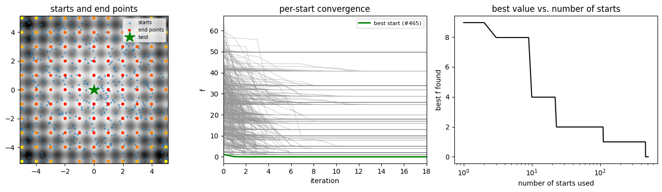
All 512 starts converged within 16 iterations (median 7), but each one only to a nearby local minimum: the end points sit on the integer grid (left panel), and the final values form discrete levels (0.995, 1.990, 3.980, …). Only one start, #465, reached the global minimum \(f = 0\) at the origin. It started at (0.235, 0.186), inside the central basin. Of the 5 starts drawn in that basin, the other 4 ended in neighbouring minima: an early L-BFGS line-search step can carry a start over a basin boundary. Because the starts are independent, the best value among the first \(S\) starts (right panel) shows what a smaller run would have found: it falls in steps as \(S\) grows, and this draw needs 466 starts before the global minimum is found.

Summary

• FORCE (and RLS) update registered readout weights from (inputs, outputs, targets); the update is a brainstate state change, so the whole training run is one for_loop.

• With forgetting factor 1, RLS reproduces ridge_regression on the samples seen so far; LMS is cheaper but slower, has a learning-rate stability limit, and keeps a noise floor at a constant learning rate.

• lasso_regression and elastic_net_regression are jit- and vmap-compatible, so a regularisation path over alpha is a single jax.vmap.

• multistart_minimize runs a local optimizer from many starts in one compiled program and reports every start’s result, iteration count and loss history, with the best start picked out.