A training loop with braintools.trainer

braintools.trainer wraps the usual training boilerplate around a brainstate model: batching, the jit-compiled gradient step, validation, callbacks, checkpoints and metric logging. Its interface follows PyTorch Lightning: the model is a LightningModule that defines what one step does, and a Trainer runs the loop.

Note

braintools.trainer is in maintenance mode. It is a lightweight training loop for small and medium models: bugs are fixed, but no new features are planned. For custom training schemes, write the loop directly with brainstate.transform and a braintools.optim optimizer (see the optimizer tutorials).

This tutorial trains a small classifier on a toy data set and covers:

1. Data: arrays wrapped in a DataLoader.

2. The model: a LightningModule with training, validation, test and prediction steps.

3. Training with EarlyStopping, ModelCheckpoint and a CSVLogger.

4. The logged curves, read back from the CSV file.

5. Reloading the best checkpoint and evaluating it on held-out data.

import os
import shutil
import tempfile

import brainstate
import jax.numpy as jnp
import matplotlib.pyplot as plt
import numpy as np
import pandas as pd

import braintools
from braintools import trainer as bt

1. Data

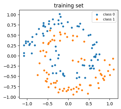
The task is to tell apart two interleaved spirals in the plane. With few training points and noisy coordinates, a flexible network can fit the training set better than it generalizes, which is what early stopping and checkpointing are for.

The labels are stored one-hot, so every sample is a pair of small arrays (x, y) with shapes (2,) and (2,). All randomness below is seeded.

def make_spirals(n_per_class, noise, rng):
    # Two interleaved spirals, scaled to about [-1, 1]^2.
    t = np.sqrt(rng.uniform(0.05, 1.0, size=(2, n_per_class))) * 3 * np.pi
    points, labels = [], []
    for c in range(2):
        angle = t[c] + c * np.pi
        xy = np.stack([t[c] * np.cos(angle), t[c] * np.sin(angle)], axis=1) / (3 * np.pi)
        points.append(xy + noise * rng.normal(size=xy.shape))
        labels.append(np.full(n_per_class, c))
    X = np.concatenate(points).astype(np.float32)
    y = np.concatenate(labels)
    order = rng.permutation(len(y))
    return X[order], y[order]


rng = np.random.default_rng(0)
X, labels = make_spirals(275, noise=0.08, rng=rng)
Y = np.eye(2, dtype=np.float32)[labels]          # one-hot targets

X_train, Y_train = X[:150], Y[:150]
X_val, Y_val = X[150:350], Y[150:350]
X_test, Y_test = X[350:], Y[350:]
print('train / val / test:', len(X_train), len(X_val), len(X_test))

fig, ax = plt.subplots(figsize=(4, 4))
for c, color in enumerate(['tab:blue', 'tab:orange']):
    m = Y_train[:, 1] == c
    ax.scatter(*X_train[m].T, s=12, color=color, label=f'class {c}')
ax.set_aspect('equal'); ax.legend(fontsize=8, loc='upper right'); ax.set_title('training set')
plt.tight_layout()

train / val / test: 150 200 200

DataLoader accepts a tuple of arrays directly (it wraps them in an ArrayDataset) and yields batches with the same structure, stacked along a new leading axis. shuffle=True with a seed reshuffles every epoch in a reproducible order.

train_loader = bt.DataLoader((X_train, Y_train), batch_size=25, shuffle=True, seed=0)
val_loader = bt.DataLoader((X_val, Y_val), batch_size=200)
test_loader = bt.DataLoader((X_test, Y_test), batch_size=200)

x_batch, y_batch = next(iter(train_loader))
print('batches per epoch:', len(train_loader), ' batch shapes:', x_batch.shape, y_batch.shape)

batches per epoch: 6  batch shapes: (25, 2) (25, 2)

2. The model

A LightningModule is a brainstate.nn.Module, so layers are declared as attributes as usual. On top of __call__ it defines the steps the trainer calls:

• training_step(batch, batch_idx) returns a dict with the 'loss' to differentiate. The trainer runs it inside brainstate.transform.grad and jit, so it must be traceable. self.log(name, value) records extra metrics; they are logged at every step.

• validation_step and test_step return a dict of metrics. The trainer averages them over the batches and adds a val_ or test_ prefix.

• predict_step returns anything; Trainer.predict collects the results.

• configure_optimizers returns a braintools.optim optimizer. Here it is SGD with momentum.

class SpiralClassifier(bt.LightningModule):
    def __init__(self, hidden=128, lr=0.02):
        super().__init__()
        self.lr = lr
        self.l1 = brainstate.nn.Linear(2, hidden)
        self.l2 = brainstate.nn.Linear(hidden, hidden)
        self.l3 = brainstate.nn.Linear(hidden, 2)

    def __call__(self, x):
        h = jnp.tanh(self.l1(x))
        h = jnp.tanh(self.l2(h))
        return self.l3(h)                      # logits

    def _loss_and_acc(self, batch):
        x, y = batch
        logits = self(x)
        loss = braintools.metric.softmax_cross_entropy(logits, y).mean()
        acc = jnp.mean(jnp.argmax(logits, -1) == jnp.argmax(y, -1))
        return loss, acc

    def training_step(self, batch, batch_idx):
        loss, acc = self._loss_and_acc(batch)
        self.log('loss', loss)
        self.log('acc', acc)
        return {'loss': loss}

    def validation_step(self, batch, batch_idx):
        loss, acc = self._loss_and_acc(batch)
        return {'loss': loss, 'acc': acc}

    def test_step(self, batch, batch_idx):
        loss, acc = self._loss_and_acc(batch)
        return {'loss': loss, 'acc': acc}

    def predict_step(self, batch, batch_idx):
        x, _ = batch
        return jnp.argmax(self(x), axis=-1)

    def configure_optimizers(self):
        return braintools.optim.SGD(lr=self.lr, momentum=0.9)

3. Training with callbacks and a CSV logger

Everything the run writes goes to a temporary directory:

• ModelCheckpoint saves a checkpoint after every validation whose val_loss is among the save_top_k=2 best seen so far (older ones are deleted), and last.ckpt at the end of the run. The file name template can use {epoch} and any metric.

• EarlyStopping stops the run once val_loss has not improved by more than min_delta for patience epochs.

• CSVLogger writes every logged metric to <save_dir>/<name>/<version>/metrics.csv, and the trainer’s hyperparameters to hparams.yaml.

enable_progress_bar=False keeps the output short. Checkpoints are saved only by a ModelCheckpoint callback; enable_checkpointing is kept for compatibility and has no effect. default_root_dir points the trainer’s own files at the temporary directory too (by default it is the current working directory).

run_dir = tempfile.mkdtemp(prefix='braintools_trainer_')

checkpoint = bt.ModelCheckpoint(
    dirpath=os.path.join(run_dir, 'checkpoints'),
    filename='epoch{epoch:03d}-val{val_loss:.4f}',
    monitor='val_loss', mode='min', save_top_k=2,
)
early_stopping = bt.EarlyStopping(monitor='val_loss', mode='min', patience=30, min_delta=1e-4)
logger = bt.CSVLogger(run_dir, name='spirals', version='run0')

brainstate.random.seed(0)
model = SpiralClassifier()
trainer = bt.Trainer(
    max_epochs=400,
    callbacks=[checkpoint, early_stopping],
    logger=logger,
    enable_progress_bar=False,
    enable_checkpointing=False,
    default_root_dir=run_dir,
    seed=0,
)
trainer.fit(model, train_loader, val_loader)

print('stopped after epoch', trainer.current_epoch, f'({trainer.global_step} steps)')
print('final metrics:', {k: round(v, 4) for k, v in trainer.callback_metrics.items()})

stopped after epoch 319 (1920 steps)
final metrics: {'train_loss': 0.0494, 'train_acc': 0.98, 'val_loss': 0.2511, 'val_acc': 0.915}

trainer.callback_metrics holds the latest epoch averages. The callbacks keep their own state: the early-stopping epoch, and the best checkpoint with its score.

print('early stopping fired at epoch:', early_stopping.stopped_epoch)
print('best val_loss:', round(float(checkpoint.best_score), 4))
print('best checkpoint:', os.path.basename(checkpoint.best_model_path))
print('checkpoint dir:', sorted(os.listdir(checkpoint.dirpath)))
print('log dir:', sorted(os.listdir(logger.log_dir)))

early stopping fired at epoch: 319
best val_loss: 0.2189
best checkpoint: epoch289-val0.2189.ckpt
checkpoint dir: ['epoch280-val0.2226.ckpt', 'epoch289-val0.2189.ckpt', 'last.ckpt']
log dir: ['hparams.yaml', 'metrics.csv']

4. The logged curves

metrics.csv has one row per training step (columns loss and acc) and one row per validation run (columns val_loss and val_acc), indexed by the global step. Each validation row is written at the step count reached at the end of its epoch.

df = pd.read_csv(logger.metrics_file_path)
print(df.shape)
df.head(10)

(2240, 5)

	step	loss	acc	val_loss	val_acc
0	0	0.603733	0.68	NaN	NaN
1	1	0.628377	0.60	NaN	NaN
2	2	0.651708	0.60	NaN	NaN
3	3	0.628534	0.56	NaN	NaN
4	4	0.721221	0.56	NaN	NaN
5	5	0.670406	0.64	NaN	NaN
6	6	NaN	NaN	0.640779	0.645
7	6	0.603613	0.64	NaN	NaN
8	7	0.668528	0.60	NaN	NaN
9	8	0.597569	0.60	NaN	NaN

n_batches = len(train_loader)
train_rows = df.dropna(subset=['loss'])
val_rows = df.dropna(subset=['val_loss'])

# Average the per-step training metrics over each epoch.
train_epoch = train_rows.groupby(train_rows['step'] // n_batches)[['loss', 'acc']].mean()
val_epoch = val_rows['step'].to_numpy() // n_batches - 1
best_epoch = int(val_epoch[np.argmin(val_rows['val_loss'].to_numpy())])

fig, axes = plt.subplots(1, 2, figsize=(10, 3.4))
axes[0].plot(train_rows['step'] / n_batches, train_rows['loss'], color='0.8', lw=0.6, label='train (per step)')
axes[0].plot(train_epoch.index, train_epoch['loss'], label='train (epoch mean)')
axes[0].plot(val_epoch, val_rows['val_loss'], label='validation')
axes[0].set_yscale('log'); axes[0].set_ylabel('cross-entropy')
axes[1].plot(train_epoch.index, train_epoch['acc'], label='train (epoch mean)')
axes[1].plot(val_epoch, val_rows['val_acc'], label='validation')
axes[1].set_ylabel('accuracy'); axes[1].set_ylim(0.4, 1.02)
for ax in axes:
    ax.axvline(best_epoch, color='k', ls='--', lw=0.8, label=f'best epoch ({best_epoch})')
    ax.set_xlabel('epoch'); ax.legend(fontsize=8)
plt.tight_layout()

print('best epoch from the CSV:', best_epoch)
print('train / val loss at the end: %.4f / %.4f' % (train_epoch['loss'].iloc[-1], val_rows['val_loss'].iloc[-1]))

best epoch from the CSV: 289
train / val loss at the end: 0.0494 / 0.2511

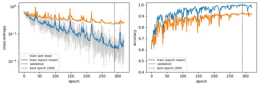
The training loss keeps falling (to 0.049 over the last epoch), while the validation loss levels off well above it from roughly epoch 200 on: with only 150 training points, the network starts fitting their noise. The lowest validation loss, 0.2189, came at epoch 289. No improvement larger than min_delta followed in the next 30 epochs (patience=30), so early stopping ended the run at epoch 319. Single steps are noisy (SGD with momentum on batches of 25 points), which is why the epoch means are drawn on top.

5. Reloading the best checkpoint

A checkpoint is a msgpack file holding the parameter values (model_state_dict), the optimizer state, the epoch, the metrics at save time and the callback states. load_checkpoint reads it as a dict:

ckpt = bt.load_checkpoint(checkpoint.best_model_path)
print(sorted(ckpt))
print('epoch:', ckpt['epoch'], ' metrics:', {k: round(float(v), 4) for k, v in ckpt['metrics'].items()})
print('parameters:', sorted(ckpt['model_state_dict']))

['callbacks', 'epoch', 'global_step', 'metrics', 'model_state_dict', 'optimizer_state_dict']
epoch: 289  metrics: {'val_acc': 0.935, 'val_loss': 0.2189}
parameters: ["('l1', 'weight')", "('l2', 'weight')", "('l3', 'weight')"]

To evaluate the best weights, build a fresh model with the same architecture and pass the checkpoint to Trainer.test(..., ckpt_path=...), which loads it before running test_step on every batch. A separate Trainer with logging off is used for evaluation, so the training run’s logs stay as they are. For comparison, the training trainer still holds the model as it was at the end of training:

final_metrics = trainer.test(dataloaders=test_loader, verbose=False)

evaluator = bt.Trainer(logger=False, enable_progress_bar=False, enable_checkpointing=False,
                       default_root_dir=run_dir)
best_model = SpiralClassifier()
best_metrics = evaluator.test(best_model, test_loader, ckpt_path=checkpoint.best_model_path, verbose=False)

print('final weights: test_loss = %.4f, test_acc = %.3f' % (final_metrics['test_loss'], final_metrics['test_acc']))
print('best weights:  test_loss = %.4f, test_acc = %.3f' % (best_metrics['test_loss'], best_metrics['test_acc']))

final weights: test_loss = 0.1624, test_acc = 0.960
best weights:  test_loss = 0.1390, test_acc = 0.965

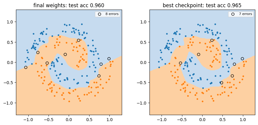
On the 200 held-out test points, the best checkpoint does a little better than the final weights: a test loss of 0.139 against 0.162, and an accuracy of 0.965 against 0.960. The gap is small because the validation loss rose only slightly after its minimum, but the checkpoint was chosen on validation data alone, without looking at the test set.

Trainer.predict returns the output of predict_step for every batch. Below, both models classify a grid of points (a single batched call per model) and the test set:

grid = np.linspace(-1.3, 1.3, 200, dtype=np.float32)
gx, gy = np.meshgrid(grid, grid)
grid_points = np.stack([gx.ravel(), gy.ravel()], axis=1)

fig, axes = plt.subplots(1, 2, figsize=(9, 4.2))
for ax, (title, m, metrics) in zip(axes, [('final weights', model, final_metrics),
                                          ('best checkpoint', best_model, best_metrics)]):
    pred_test = np.concatenate(evaluator.predict(m, test_loader))
    region = np.asarray(jnp.argmax(m(grid_points), axis=-1)).reshape(gx.shape)
    ax.contourf(gx, gy, region, levels=[-0.5, 0.5, 1.5], colors=['#c6dbef', '#fdd0a2'])
    wrong = pred_test != Y_test.argmax(1)
    ax.scatter(*X_test[~wrong].T, s=8, c=np.where(Y_test[~wrong, 1] == 1, 'tab:orange', 'tab:blue'))
    ax.scatter(*X_test[wrong].T, s=40, facecolors='none', edgecolors='k', label=f'{wrong.sum()} errors')
    ax.set_title(f"{title}: test acc {metrics['test_acc']:.3f}")
    ax.set_aspect('equal'); ax.legend(loc='upper right', fontsize=8)
plt.tight_layout()

Finally, remove the run directory:

shutil.rmtree(run_dir)
print(os.path.exists(run_dir))

False

Summary

• A LightningModule defines training_step (traced under jit and grad, logs with self.log), validation_step / test_step (return metric dicts that the trainer averages and prefixes) and configure_optimizers.

• DataLoader batches plain arrays; give it a seed when shuffling.

• ModelCheckpoint keeps the save_top_k best checkpoints by a monitored metric plus last.ckpt; EarlyStopping ends the run when that metric stalls; CSVLogger writes a metrics.csv that pandas reads directly.

• Trainer.test(model, loader, ckpt_path=...) (and validate / predict) evaluates a fresh model from a saved checkpoint.

For anything beyond this loop (custom update rules, online learning, multi-optimizer schemes) drive the model directly with brainstate.transform and the braintools.optim optimizers; see the optimization tutorials.