Local Field Potential Analysis

This tutorial covers the LFP tools of braintools.analysis: generating an LFP from spikes, and the spectral, coupling, and laminar analyses. unitary_LFP and current_source_density are in braintools.analysis.field; the spectral and coupling measures are in braintools.analysis.spectral. Each analysis is first checked on a synthetic signal whose answer is known.

Function	Purpose
unitary_LFP(times, spikes, spike_type, location=...)	kernel-based LFP contribution of an excitatory or inhibitory population
power_spectral_density(lfp, dt, nperseg=None, ...)	Welch power spectrum
coherence_analysis(x, y, dt, nperseg=None, ...)	magnitude-squared coherence (Welch)
spectral_entropy(lfp, dt, freq_range=(1, 100))	normalized entropy of the spectrum, 0 (one peak) to 1 (flat)
phase_amplitude_coupling(lfp, dt, phase_freq_range, amplitude_freq_range, n_bins=18)	Tort modulation index
theta_gamma_coupling(lfp, dt)	the same with 4-8 Hz phase and 30-80 Hz amplitude
lfp_phase_coherence(signals, dt, freq_band)	pairwise phase-locking value between channels in a band
current_source_density(lfp_laminar, electrode_spacing)	second spatial difference of a laminar recording

For the spectral functions, dt is the sampling interval: a plain number is in seconds, and a quantity is converted. unitary_LFP takes times in milliseconds.

1. Setup

import brainunit as u
import jax.numpy as jnp
import matplotlib.pyplot as plt
import numpy as np

import braintools.analysis as ba

rng = np.random.default_rng(0)

2. An LFP from Spiking Activity

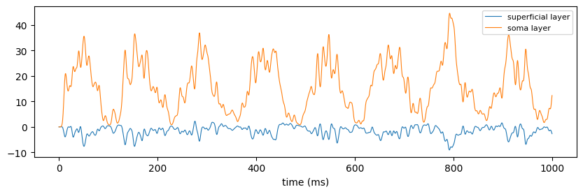
unitary_LFP places the neurons of a population at random in a 0.2 mm x 0.2 mm area around the electrode. Each spike adds a Gaussian waveform whose amplitude decays with distance and whose delay grows with distance (axonal conduction). The amplitude and sign of the excitatory and inhibitory contributions depend on the recording location ('soma layer', 'deep layer', 'superficial layer', 'surface layer').

Below, 200 excitatory and 50 inhibitory neurons fire with a rate modulated at 8 Hz (theta) for 10 s.

dt_ms = 0.5
T = int(10_000 / dt_ms)
t_ms = np.arange(T) * dt_ms
rate = 10 * (1 + 0.8 * np.sin(2 * np.pi * 8 * t_ms / 1000))  # Hz
exc = (rng.random((T, 200)) < (rate * dt_ms * 1e-3)[:, None]).astype(float)
inh = (rng.random((T, 50)) < (2 * rate * dt_ms * 1e-3)[:, None]).astype(float)

lfps = {}
for location in ["superficial layer", "soma layer"]:
    e = np.asarray(ba.field.unitary_LFP(t_ms, exc, "exc", location=location, seed=0))
    i = np.asarray(ba.field.unitary_LFP(t_ms, inh, "inh", location=location, seed=0))
    lfps[location] = e + i
    print(f"{location:17s}: correlation of E and I contributions {np.corrcoef(e, i)[0, 1]:+.2f}")

fig, ax = plt.subplots(figsize=(10, 2.8))
for location, x in lfps.items():
    ax.plot(t_ms[:2000], x[:2000], lw=0.8, label=location)
ax.set_xlabel("time (ms)")
ax.legend(fontsize=8)
plt.show()

lfp = lfps["soma layer"]
dt = dt_ms * u.ms

superficial layer: correlation of E and I contributions -0.79

soma layer       : correlation of E and I contributions +0.79

3. Power Spectrum and Frequency Resolution

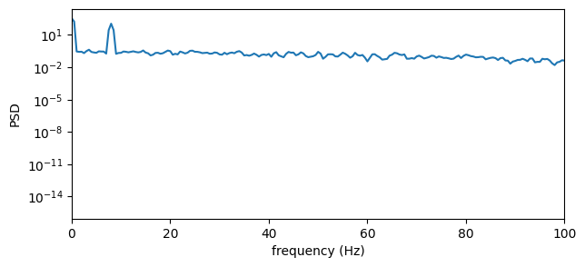
power_spectral_density uses Welch’s method: the signal is cut into Hann-windowed segments of nperseg samples with 50 % overlap, and their periodograms are averaged. The frequency resolution is \(1 / (\texttt{nperseg} \cdot dt)\). The default nperseg = n_time // 8 is fine for long recordings but too coarse for short ones, so set it from the resolution you need: 2 s segments give 0.5 Hz bins.

The result equals scipy.signal.welch with the same (symmetric) Hann window and detrend=False; scipy’s defaults differ slightly (a periodic window and mean detrending).

from scipy import signal as sps

freqs, psd = ba.spectral.power_spectral_density(lfp, dt, nperseg=4000)
f_ref, p_ref = sps.welch(lfp, fs=1000 / dt_ms, window=np.hanning(4000), nperseg=4000, detrend=False)
print(f"resolution {float(freqs[1]):.2f} Hz; max relative difference from scipy {np.max(np.abs(np.asarray(psd) - p_ref)) / p_ref.max():.1e}")
print(f"spectral peak at {float(freqs[np.argmax(np.asarray(psd)[2:]) + 2]):.1f} Hz (rate modulation 8 Hz)")


def band_power(freqs, psd, lo, hi):
    f, p = np.asarray(freqs), np.asarray(psd)
    m = (f >= lo) & (f < hi)
    return p[m].sum() * (f[1] - f[0])


total = band_power(freqs, psd, 1, 100)
for name, (lo, hi) in {"delta": (1, 4), "theta": (4, 12), "beta": (12, 30), "gamma": (30, 100)}.items():
    print(f"  {name:6s} {100 * band_power(freqs, psd, lo, hi) / total:5.1f} % of 1-100 Hz power")

fig, ax = plt.subplots(figsize=(7, 3))
ax.semilogy(freqs, psd)
ax.set_xlim(0, 100)
ax.set_xlabel("frequency (Hz)")
ax.set_ylabel("PSD")
plt.show()

resolution 0.50 Hz; max relative difference from scipy 9.1e-08
spectral peak at 8.0 Hz (rate modulation 8 Hz)
  delta    0.9 % of 1-100 Hz power
  theta   86.6 % of 1-100 Hz power
  beta     4.4 % of 1-100 Hz power
  gamma    8.1 % of 1-100 Hz power

4. Coherence

coherence_analysis estimates \(C_{xy}(f) = \lvert\langle P_{xy}\rangle\rvert^2 / (\langle P_{xx}\rangle\langle P_{yy}\rangle)\) by averaging over Welch segments; with a single segment it would be 1 everywhere, so make sure many segments fit. For two signals that share a component \(s\) plus independent noise of equal power, \(x = s + n_1\), \(y = s + n_2\), the true coherence is \(\left(S / (S + N)\right)^2\) , where \(S\) and \(N\) are the signal and noise spectra. The Welch estimate is biased upward by roughly \((1 - C)/K\) for \(K\) averaged segments, which matters where the true coherence is small.

fs = 1000.0
n = 60_000
shared = np.sin(2 * np.pi * 10 * np.arange(n) / fs) + rng.normal(size=n) * 0.5
x = shared + rng.normal(size=n)
y = shared + rng.normal(size=n)
f, coh = ba.spectral.coherence_analysis(x, y, 1 / fs, nperseg=2000)
f, coh = np.asarray(f), np.asarray(coh)

S_noise = 0.25 / (fs / 2)  # one-sided PSD of the shared white noise (variance 0.25)
N = 1.0 / (fs / 2)  # one-sided PSD of each private noise (variance 1)
print(f"coherence at 10 Hz (shared sinusoid): {coh[np.argmin(np.abs(f - 10))]:.3f}")
K = 2 * n // 2000 - 1  # number of 50 %-overlapping segments
C = (S_noise / (S_noise + N)) ** 2
print(f"coherence elsewhere (shared noise only): mean {coh[(f > 20) & (f < 400)].mean():.3f}; "
      f"true value {C:.3f}, plus estimator bias (1 - C)/K = {(1 - C) / K:.3f} -> {C + (1 - C) / K:.3f}")

coherence at 10 Hz (shared sinusoid): 0.994
coherence elsewhere (shared noise only): mean 0.061; true value 0.040, plus estimator bias (1 - C)/K = 0.016 -> 0.056

5. Spectral Entropy

spectral_entropy normalizes the power spectrum in freq_range to a probability distribution and returns its Shannon entropy divided by the maximum (log of the number of bins): close to 1 for white noise and close to 0 for a single sharp peak.

t = np.arange(20_000) / fs
signals = {
    "white noise": rng.normal(size=t.size),
    "10 Hz sine + 1% noise": np.sin(2 * np.pi * 10 * t) + 0.01 * rng.normal(size=t.size),
    "simulated LFP": None,
}
for name, sig in signals.items():
    h = ba.spectral.spectral_entropy(lfp, dt) if sig is None else ba.spectral.spectral_entropy(sig, 1 / fs)
    print(f"{name:22s} spectral entropy {float(h):.3f}")

white noise            spectral entropy 0.994
10 Hz sine + 1% noise  spectral entropy 0.158

simulated LFP          spectral entropy 0.380

6. Phase-Amplitude Coupling

phase_amplitude_coupling extracts the phase of a slow band and the amplitude envelope of a fast band (analytic signals via an FFT band-pass), averages the amplitude in n_bins phase bins, and returns Tort’s modulation index: the Kullback-Leibler divergence of that amplitude distribution from uniform, divided by \(\log(\texttt{n\_bins})\). It also returns the bin centres and mean amplitudes.

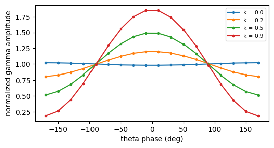
The index is small in practice: even strong coupling gives values of a few hundredths. Calibrate it with synthetic signals before interpreting a measurement. Here theta (6 Hz) modulates the amplitude of a 60 Hz oscillation with depth \(k\):

t = np.arange(20_000) / fs
theta = np.sin(2 * np.pi * 6 * t)
print(f"{'depth k':>8s} {'MI':>9s} {'theta_gamma_coupling':>21s}")
results = {}
for k in [0.0, 0.2, 0.5, 0.9]:
    sig = theta + (1 + k * theta) * 0.5 * np.sin(2 * np.pi * 60 * t) + 0.3 * rng.normal(size=t.size)
    mi, bins, amps = ba.spectral.phase_amplitude_coupling(sig, 1 / fs, phase_freq_range=(4, 8), amplitude_freq_range=(50, 70))
    results[k] = (bins, amps)
    print(f"{k:8.1f} {float(mi):9.5f} {float(ba.spectral.theta_gamma_coupling(sig, 1 / fs)):21.5f}")

fig, ax = plt.subplots(figsize=(6, 3))
for k, (bins, amps) in results.items():
    ax.plot(np.degrees(bins), np.asarray(amps) / np.mean(amps), "o-", ms=3, label=f"k = {k}")
ax.set_xlabel("theta phase (deg)")
ax.set_ylabel("normalized gamma amplitude")
ax.legend(fontsize=8)
plt.show()

mi_lfp, _, _ = ba.spectral.phase_amplitude_coupling(lfp, dt)
print(f"simulated LFP: MI {float(mi_lfp):.5f}")

 depth k        MI  theta_gamma_coupling

     0.0   0.00003               0.00006
     0.2   0.00339               0.00320
     0.5   0.02195               0.02066
     0.9   0.07078               0.06335

simulated LFP: MI 0.01374

For no coupling the index is close to 0 but not exactly 0 (finite data); compare with surrogates, for example by shifting the amplitude series relative to the phase series, to judge significance. The simulated LFP has no gamma rhythm, yet its index is clearly non-zero: the spike waveforms contribute broadband high-frequency power, and that power rises and falls with the theta-modulated firing rate. This is genuine phase-amplitude coupling, which is why a non-zero index alone does not prove a nested oscillation.

7. Phase Coherence Across Channels

lfp_phase_coherence(signals, dt, freq_band) band-passes every channel, takes its instantaneous phase, and returns the matrix of pairwise phase-locking values \(\lvert\langle e^{i(\phi_i - \phi_j)}\rangle_t\rvert\), which is 1 for a constant phase difference regardless of its value. Channels that carry no power in the band are reported as 0 rather than an arbitrary phase.

alpha = np.sin(2 * np.pi * 10 * t)
channels = np.stack([
    alpha + 0.5 * rng.normal(size=t.size),
    np.roll(alpha, 25) + 0.5 * rng.normal(size=t.size),  # 90 degree lag at 10 Hz
    -alpha + 0.5 * rng.normal(size=t.size),  # anti-phase
    rng.normal(size=t.size),  # unrelated
], axis=1)
plv = np.asarray(ba.spectral.lfp_phase_coherence(channels, 1 / fs, freq_band=(8, 12)))
print(np.round(plv, 3))

[[1.    0.998 0.998 0.076]
 [0.998 1.    0.998 0.076]
 [0.998 0.998 1.    0.081]
 [0.076 0.076 0.081 1.   ]]

Channels 0-2 lock to each other at different but constant phase differences (0, 90 and 180 degrees) and all give a PLV near 1. The unrelated channel is low but not 0: for independent signals the PLV has a finite-data floor of roughly \(1/\sqrt{\text{duration} \times \text{bandwidth}}\) (here \(1/\sqrt{20\,\text{s} \times 4\,\text{Hz}} \approx 0.1\)).

8. Current Source Density

For a laminar recording with electrode spacing \(h\), current_source_density returns

\[\text{CSD}_k = -\sigma\,\frac{V_{k+1} - 2V_k + V_{k-1}}{h^2},\]

the negative second spatial difference along the electrode axis (the last axis by default), scaled by the conductivity conductivity (default 1). The two boundary electrodes are dropped. Negative CSD is a current sink and positive a source. A potential trough at a depth therefore appears as a sink flanked by sources:

h = 0.05  # mm
depth = np.arange(20) * h
z0, s = 0.5, 0.08
profile = -np.exp(-(depth - z0) ** 2 / (2 * s ** 2))  # a potential trough at 0.5 mm
V = profile[None, :] * np.sin(2 * np.pi * 8 * t[:200])[:, None]  # (time, electrodes), oscillating amplitude

csd = np.asarray(ba.field.current_source_density(V, h))
exact = -(np.exp(-(depth - z0) ** 2 / (2 * s ** 2)) * ((depth - z0) ** 2 / s ** 4 - 1 / s ** 2)) * -1  # -d2V/dz2
print(f"CSD shape {csd.shape} (two boundary electrodes dropped)")
peak = np.argmax(np.abs(V).max(axis=1))
print(f"at the trough depth: CSD {csd[peak, 9]:.1f}, analytic -V'' {exact[10] * np.sin(2 * np.pi * 8 * t[peak]):.1f}")

fig, axes = plt.subplots(1, 2, figsize=(10, 3.2), sharey=True)
axes[0].plot(V[peak], depth)
axes[0].set_title("potential at peak time")
axes[0].set_ylabel("depth (mm)")
axes[1].plot(csd[peak], depth[1:-1], "o-", ms=3, label="current_source_density")
axes[1].plot(exact * np.sin(2 * np.pi * 8 * t[peak]), depth, "--", label="analytic")
axes[1].axvline(0, color="0.6", lw=0.8)
axes[1].set_title("CSD (negative = sink)")
axes[1].legend(fontsize=8)
axes[0].invert_yaxis()
fig.tight_layout()
plt.show()

CSD shape (200, 18) (two boundary electrodes dropped)
at the trough depth: CSD -141.9, analytic -V'' -156.2

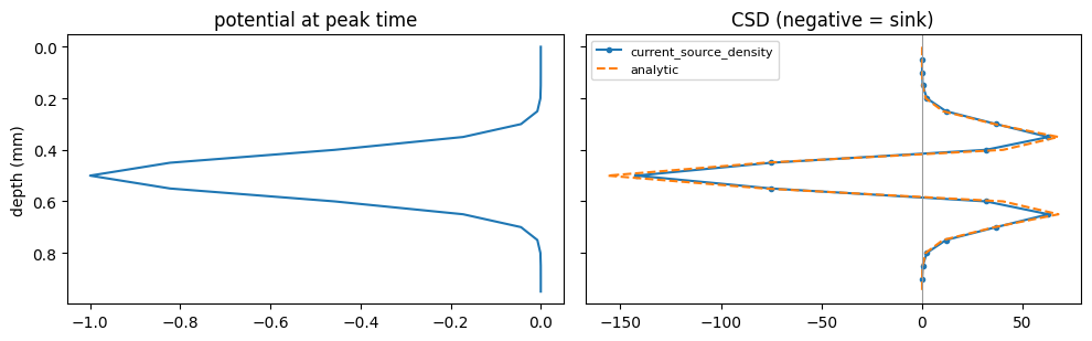
The 3-point difference slightly underestimates the analytic second derivative when the spacing is not small compared with the width of the profile (here \(h = 0.05\) mm against \(\sigma = 0.08\) mm).

Summary

• unitary_LFP turns population spikes into an LFP whose shape depends on the recording location.

• Choose nperseg from the frequency resolution you need (\(1/(\texttt{nperseg}\cdot dt)\)); the default is too coarse for short recordings. Results equal scipy.signal.welch / coherence with the same window and no detrending.

• Coherence needs many segments; spectral entropy runs from 0 (peaked) to 1 (flat).

• Tort’s modulation index is small even for strong coupling: calibrate with synthetic signals and test against surrogates.

• lfp_phase_coherence is a phase-locking value in a band; current_source_density is \(-\sigma\,\partial^2 V/\partial z^2\) with sinks negative.