Fitting models to data

This tutorial fits dynamical models to data with braintools.fit. The data are simulated from models with known parameters, so every fit can be checked against the truth:

1. Simulate a Hopf (Stuart–Landau) oscillator with braintools.quad.odeint (fixed step) and solve_ivp (adaptive step).

2. Fit its bifurcation parameter and frequency with a Fitter and a composed Objective, from 8 starting points minimised at once.

3. Check the fit: the loss landscape with fit.sweep, and confidence intervals with fit.hessian_ci.

4. Fit a module: recover the couplings of a Wilson–Cowan model written as a brainstate module with brainstate.nn.Param parameters.

5. Losses for spiking data, and saving results to HDF5.

import os
import tempfile

import brainstate
import jax
import jax.numpy as jnp
import matplotlib.pyplot as plt
import numpy as np

from braintools import fit, quad
from braintools.fit import Fitter, Term, losses

1. Simulating trajectories

The Stuart–Landau oscillator is the normal form of a Hopf bifurcation:

\[\dot x = (a - x^2 - y^2)\,x - \omega y, \qquad \dot y = (a - x^2 - y^2)\,y + \omega x.\]

For \(a > 0\) the trajectory settles on a limit cycle of radius \(\sqrt a\) that rotates at angular frequency \(\omega\). quad.odeint(f, y0, t0, t1, dt, *args) integrates it with any registered stepper (method='rk4' by default) as one compiled scan, and returns the time grid and the stacked states. Extra positional arguments are passed through to f.

def hopf(y, t, a, omega):
    x, v = y
    r2 = x * x + v * v
    return (a - r2) * x - omega * v, (a - r2) * v + omega * x

y0 = (jnp.asarray(0.5), jnp.asarray(0.0))
ts, (xs, vs) = quad.odeint(hopf, y0, 0.0, 10.0, 0.05, 0.8, 1.5)
print(ts.shape, xs.shape)

(201,) (201,)

quad.solve_ivp integrates the same system with an adaptive step size (Dormand–Prince 5(4) with a PI step-size controller). With t_eval it returns the solution at the requested times; here the two solvers agree to within a few \(10^{-6}\):

sol = quad.solve_ivp(hopf, (0.0, 10.0), y0, 0.8, 1.5, rtol=1e-8, atol=1e-10, t_eval=ts)
print('accepted steps:', int(sol.n_steps), ' rejected:', int(sol.n_rejected), ' success:', bool(sol.success))
print('max |odeint - solve_ivp| =', float(jnp.max(jnp.abs(sol.ys[0] - xs))))

accepted steps: 295  rejected: 96  success: True
max |odeint - solve_ivp| = 2.8461217880249023e-06

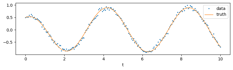
The observed data are the \(x\) trace with measurement noise. The truth is \(a = 0.8\), \(\omega = 1.5\).

truth = {'a': 0.8, 'omega': 1.5}

def simulate(params):
    _, (x, _) = quad.odeint(hopf, y0, 0.0, 10.0, 0.05, params['a'], params['omega'])
    return x

noise = 0.05 * jax.random.normal(jax.random.PRNGKey(1), xs.shape)
data = simulate(truth) + noise

plt.figure(figsize=(8, 2.5))
plt.plot(ts, data, '.', ms=3, label='data')
plt.plot(ts, simulate(truth), lw=1, label='truth')
plt.xlabel('t'); plt.legend(); plt.tight_layout()

2. Fitting with a Fitter

A fit needs three things:

• a pure simulate(params) function of a dict of parameters;

• an objective objective(prediction, target) -> scalar;

• a search space {name: (low, high)}.

Objectives compose from Terms with + and scalar *. Here the loss is the mean squared error plus a small correlation term, which rewards getting the phase right even when the amplitude is off. Objective.breakdown reports each term:

objective = Term(losses.mse, name='mse') + 0.1 * Term(losses.correlation_loss, name='corr')
print(objective)
print({k: round(float(v), 4) for k, v in objective.breakdown(simulate(truth), data).items()})

Objective(1.0*mse + 0.1*corr)

{'mse': 0.0029, 'corr': 0.0004}

Fitter.fit(target, n_starts=8, key=...) draws 8 starting points uniformly inside the bounds and minimises all of them at once: the default 'grad' backend runs L-BFGS on every start inside one compiled, vmapped loop. Each bounded parameter is optimised in an unconstrained space through a sigmoid, so the iterates always stay inside the box.

space = {'a': (0.2, 2.0), 'omega': (0.5, 3.0)}
fitter = Fitter(simulate, objective, space)
res = fitter.fit(data, n_starts=8, key=jax.random.PRNGKey(0), n_steps=200)

print(res)
print({k: round(float(v), 4) for k, v in res.best_params.items()}, ' truth:', truth)
print('final loss per start:', np.round(np.asarray(res.losses), 4))

FitResult(backend='grad', best_loss=0.00329198, n_starts=8, params=[a, omega])
{'a': 0.7886, 'omega': 1.5008}  truth: {'a': 0.8, 'omega': 1.5}
final loss per start: [0.5226 0.5167 0.0033 0.0033 0.0033 0.0033 0.5167 0.5109]

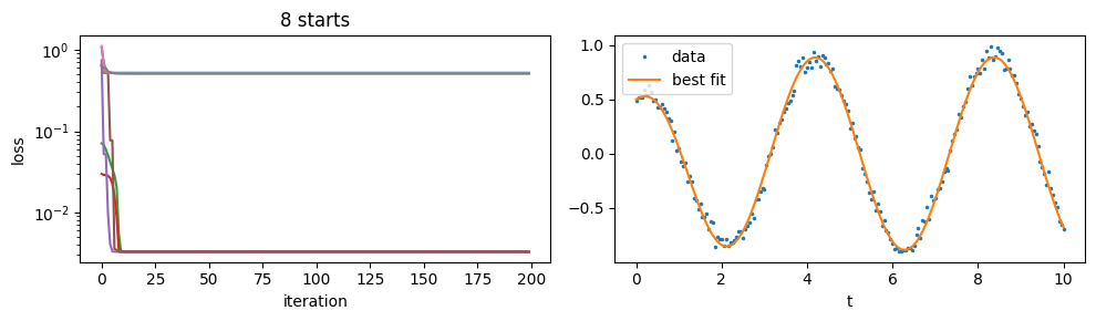
The final losses show why several starts are needed. Every start that ends at loss ≈ 0.003, the floor set by the measurement noise (variance \(0.05^2 = 0.0025\)), found the truth. The others end near 0.52: with the wrong frequency, the best they can do is shrink the oscillation, so they run to the lower bound of \(a\). res.history holds the loss of every start at every iteration:

fig, axes = plt.subplots(1, 2, figsize=(10, 3))
axes[0].semilogy(np.asarray(res.history).T)
axes[0].set_xlabel('iteration'); axes[0].set_ylabel('loss'); axes[0].set_title('8 starts')
axes[1].plot(ts, data, '.', ms=3, label='data')
axes[1].plot(ts, simulate(res.best_params), lw=1.5, label='best fit')
axes[1].set_xlabel('t'); axes[1].legend()
plt.tight_layout()

3. Checking the fit

The loss landscape

fit.sweep(fn, grid) evaluates a pure function over a parameter grid. mode='product' evaluates the cartesian product, and batch_size evaluates the points in vmapped chunks, so memory stays bounded. Here it maps the loss over 60 × 60 values of \((a, \omega)\):

grid = {'a': jnp.linspace(0.2, 2.0, 60), 'omega': jnp.linspace(0.5, 3.0, 60)}
landscape, table = fit.sweep(lambda p: objective(simulate(p), data), grid, batch_size=400)
print(landscape.shape)

plt.figure(figsize=(5, 3.5))
plt.pcolormesh(grid['omega'], grid['a'], jnp.log10(landscape), shading='auto')
plt.colorbar(label='log10 loss')
starts = res.params
plt.plot(starts['omega'], starts['a'], 'wo', ms=5, mec='k', label='end points of the 8 starts')
plt.plot(truth['omega'], truth['a'], 'r*', ms=12, label='truth')
plt.xlabel('omega'); plt.ylabel('a'); plt.legend(fontsize=7, loc='upper right'); plt.tight_layout()

(60, 60)

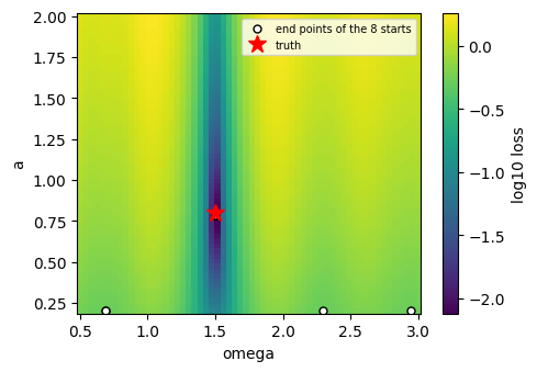
The loss has one narrow valley at the true frequency and is almost flat elsewhere. A start whose \(\omega\) lies outside the valley gets almost no gradient towards it, so it lowers the loss by shrinking the amplitude instead and ends at the lower bound of \(a\) (the white dots). Several starts make it likely that at least one begins inside the valley.

Confidence intervals

fit.hessian_ci turns the curvature of the loss at the optimum into confidence intervals. With kind='sse', the loss is a sum of squared residuals over n_data points. For a linear model these are exactly the ordinary-least-squares intervals. Here the 95% intervals are narrow and contain the truth:

sse = lambda p: jnp.sum((simulate(p) - data) ** 2)
ci = fit.hessian_ci(sse, res.best_params, kind='sse', n_data=data.size)
for name in ('a', 'omega'):
    print(f"{name:6s} {float(ci.estimate[name]):.4f} ± {float(ci.stderr[name]):.4f}   "
          f"95% CI [{float(ci.low[name]):.4f}, {float(ci.high[name]):.4f}]   truth {truth[name]}")

a      0.7886 ± 0.0100   95% CI [0.7688, 0.8083]   truth 0.8
omega  1.5008 ± 0.0010   95% CI [1.4988, 1.5027]   truth 1.5

4. Fitting a brainstate module

Models are usually written as brainstate modules. Fitter.from_module(model, predict, objective) fits every brainstate.nn.Param with fit=True (the default). Each parameter’s own transform, here SigmoidT(5, 20), sets its bounds.

During the fit the model is not modified. The best values are written back into the parameters only when fit returns.

The model is a two-population Wilson–Cowan network driven by a slow sinusoid; we recover the excitatory-to-excitatory and inhibitory-to-excitatory couplings from the simulated rates.

def sigmoid(x, gain, theta):
    return 1. / (1. + jnp.exp(-gain * (x - theta)))


class WilsonCowan(brainstate.nn.Module):
    def __init__(self, w_ee, w_ei):
        super().__init__()
        self.w_ee = brainstate.nn.Param(w_ee, t=brainstate.nn.SigmoidT(5., 20.))
        self.w_ei = brainstate.nn.Param(w_ei, t=brainstate.nn.SigmoidT(5., 20.))
        self.w_ie, self.w_ii = 13., 11.

    def rhs(self, y, t, w_ee, w_ei):
        e, i = y
        drive = 1.5 + jnp.sin(0.5 * t)
        de = -e + sigmoid(w_ee * e - w_ei * i + drive, 1.3, 4.)
        di = (-i + sigmoid(self.w_ie * e - self.w_ii * i, 2., 3.7)) / 2.
        return de, di

    def rates(self):
        y0 = (jnp.asarray(0.1), jnp.asarray(0.05))
        _, (e, i) = quad.odeint(self.rhs, y0, 0.0, 40.0, 0.1, self.w_ee.value(), self.w_ei.value())
        return jnp.stack([e, i], axis=-1)


target = WilsonCowan(16., 12.).rates()
model = WilsonCowan(10., 8.)          # wrong initial couplings
res_wc = Fitter.from_module(model, lambda m: m.rates(), losses.mse).fit(
    target, n_starts=8, key=jax.random.PRNGKey(0), n_steps=200)
print({k: round(float(v), 3) for k, v in res_wc.best_params.items()}, ' truth: w_ee=16, w_ei=12')
print('written back to the model:', round(float(model.w_ee.value()), 3), round(float(model.w_ei.value()), 3))

{'w_ee': 16.0, 'w_ei': 12.0}  truth: w_ee=16, w_ei=12
written back to the model: 16.0 12.0

The other backends take the same problem. backend='scipy' runs scipy.optimize.minimize from each start with jit-compiled gradients. backend='nevergrad' runs a gradient-free evolutionary search that evaluates each generation as one vmapped batch. Here is SciPy’s L-BFGS-B on the Hopf fit:

res_scipy = Fitter(simulate, objective, space, backend='scipy').fit(
    data, n_starts=8, key=jax.random.PRNGKey(0), n_steps=200)
print(res_scipy.backend, {k: round(float(v), 4) for k, v in res_scipy.best_params.items()})

scipy {'a': 0.7886, 'omega': 1.5008}

5. Losses for spiking data, and saving results

braintools.fit.losses also compares spiking activity:

• rate_loss compares mean firing rates;

• cv_loss compares ISI irregularity;

• van_rossum_loss gives the van Rossum distance between dense rasters. It is differentiable, so gradients flow through surrogate-gradient spikes.

Each loss’s docstring states whether it is differentiable.

from braintools import surrogate

dt = 0.1
t = jnp.arange(2000) * dt                                          # 200 ms
target_raster = (jnp.sin(2 * jnp.pi * t / 25.0)[:, None] > 0.995).astype(float) * jnp.ones((1, 3))

def raster(shift):
    # a surrogate spike: Heaviside forward, sigmoid gradient backward
    return surrogate.sigmoid(jnp.sin(2 * jnp.pi * (t[:, None] - shift) / 25.0) - 0.995) * jnp.ones((1, 3))

loss = lambda s: losses.van_rossum_loss(raster(s), target_raster, tau=5.0, dt=dt)
print('loss at shift 0, 2 ms:', round(float(loss(0.0)), 4), round(float(loss(2.0)), 4))
print('d loss / d shift at 2 ms:', round(float(jax.grad(loss)(2.0)), 4))
print('rate loss:', float(losses.rate_loss(raster(2.0), target_raster, dt=dt)))

loss at shift 0, 2 ms: 0.0 5.3243

d loss / d shift at 2 ms: 2.3121
rate loss: 0.0

braintools.file.save_hdf5 stores nested dicts of arrays, brainunit quantities and SpikeTrains (with the hdf5 extra, pip install braintools[hdf5]). It is a convenient format for fit results. NWB and NEO exporters for spike data are in the same module.

from braintools.file import load_hdf5, save_hdf5

path = os.path.join(tempfile.mkdtemp(), 'hopf_fit.h5')
save_hdf5(path, {'best_params': res.best_params, 'losses': res.losses, 'history': res.history,
                 'ci_low': ci.low, 'ci_high': ci.high})
loaded = load_hdf5(path)
print(sorted(loaded), {k: round(float(v), 4) for k, v in loaded['best_params'].items()})

['best_params', 'ci_high', 'ci_low', 'history', 'losses'] {'a': 0.7886, 'omega': 1.5008}

Summary

Task	API
trajectories	quad.odeint (fixed step, checkpoint=True for long backprop), quad.solve_ivp (adaptive)
objectives	fit.Term, fit.Objective, fit.losses.*
fitting	fit.Fitter (functional) and Fitter.from_module; backends 'grad', 'scipy', 'nevergrad'
many starts of any pure function	optim.multistart_minimize, optim.multistart_init
exploration and uncertainty	fit.sweep, fit.hessian_ci
data formats	file.save_hdf5/load_hdf5, NWB (save_nwb_units, …) and NEO (to_neo, from_neo)

See the API reference for every parameter.