

Trajectories and adaptive integration#
The ODE tutorial advances a state one step at a time with the ode_*_step functions. To get a whole trajectory, braintools.quad has two drivers:
quad.odeint(f, y0, t0, t1, dt, *args, method=...)runs any registered fixed-step stepper over a uniform time grid as one compiledscan;quad.solve_ivp(f, (t0, t1), y0, *args, method='dopri5', rtol=..., atol=..., t_eval=...)adapts the step size to meet an error tolerance, likescipy.integrate.solve_ivp.
Both are differentiable and work under jit and vmap. This tutorial covers:
odeintwith fixed-step methods, and how their accuracy scales with the step size;solve_ivpon the stiff-ish Van der Pol oscillator, checked against SciPy, with and withoutt_eval;gradients through both drivers (
checkpoint=True), used for a parameter sensitivity;the method registry:
list_methods,get_methodandregister_methodwith a custom stepper.
import time

import brainstate
import jax
import jax.numpy as jnp
import matplotlib.pyplot as plt
import numpy as np
import scipy.integrate

from braintools import quad

jax.config.update('jax_enable_x64', True)  # float64, to compare errors down to 1e-10
1. Fixed-step trajectories with odeint#
The harmonic oscillator \(\ddot x = -\omega^2 x\) has the exact solution \(x(t) = \cos \omega t\), \(v(t) = -\omega \sin \omega t\) for \(x(0) = 1\), \(v(0) = 0\). The right-hand side takes the state first and the time second, f(y, t, *args) (SciPy uses (t, y)). Extra positional arguments after dt are passed on to f.
def oscillator(y, t, omega):
    x, v = y
    return jnp.stack([v, -omega ** 2 * x])


omega, T = 2.0, 10.0
y0 = jnp.array([1.0, 0.0])

ts, ys = quad.odeint(oscillator, y0, 0.0, T, 0.05, omega, method='rk4')
print('ts:', ts.shape, ' ys:', ys.shape, ' ys[0] == y0:', bool(jnp.all(ys[0] == y0)))

ts_s, ys_s = quad.odeint(oscillator, y0, 0.0, T, 0.05, omega, method='rk4', save_every=10)
print('save_every=10 -> ts:', ts_s.shape, ' first times:', ts_s[:3])
ts: (201,) ys: (201, 2) ys[0] == y0: True
save_every=10 -> ts: (21,) first times: [0. 0.5 1. ]
ts holds the n + 1 = 201 grid times including t0, and every leaf of ys gains a leading time axis. save_every=10 keeps one state in ten, which saves memory on long runs without changing the steps.
method selects the stepper by name. Below, the forward Euler (order 1), midpoint ('rk2', order 2) and classical Runge–Kutta ('rk4', order 4) methods integrate the oscillator to \(T = 10\) with step sizes from 0.04 down to 0.0025. The left panel shows trajectories at dt = 0.05, the right panel the final-time error. Looping over a few configurations in Python is fine; each odeint call is one compiled scan over the time steps.
exact_T = jnp.array([jnp.cos(omega * T), -omega * jnp.sin(omega * T)])
dts = np.array([0.04, 0.02, 0.01, 0.005, 0.0025])
methods = ['euler', 'rk2', 'rk4']

errors = {}
for m in methods:
    errors[m] = np.array([float(jnp.max(jnp.abs(quad.odeint(oscillator, y0, 0.0, T, dt, omega, method=m)[1][-1]
                                               - exact_T)))
                          for dt in dts])
    orders = np.log2(errors[m][:-1] / errors[m][1:])
    print(f'{m:6s} errors {np.array2string(errors[m], precision=2)}  observed order {np.round(orders, 2)}')

fig, axes = plt.subplots(1, 2, figsize=(12, 4))
t_fine = np.linspace(0, T, 1000)
axes[0].plot(t_fine, np.cos(omega * t_fine), 'k', lw=3, alpha=0.3, label='exact')
for m in methods:
    ts_m, ys_m = quad.odeint(oscillator, y0, 0.0, T, 0.05, omega, method=m)
    axes[0].plot(ts_m, ys_m[:, 0], lw=1, label=m)
axes[0].set_xlabel('t')
axes[0].set_ylabel('x(t)')
axes[0].set_title('dt = 0.05')
axes[0].legend(loc='lower left')
for m, order in zip(methods, [1, 2, 4]):
    axes[1].loglog(dts, errors[m], 'o-', label=m)
    axes[1].loglog(dts, errors[m][-1] * (dts / dts[-1]) ** order, 'k:', lw=0.8)
axes[1].set_xlabel('dt')
axes[1].set_ylabel('max error at t = 10')
axes[1].set_title('convergence (dotted: slopes 1, 2, 4)')
axes[1].legend()
plt.tight_layout()
plt.show()
euler errors [2.15 0.88 0.4 0.19 0.09] observed order [1.28 1.14 1.07 1.03]
rk2 errors [1.93e-02 4.81e-03 1.21e-03 3.03e-04 7.60e-05] observed order [2.01 1.99 2. 2. ]
rk4 errors [6.39e-06 3.83e-07 2.42e-08 1.52e-09 9.49e-11] observed order [4.06 3.99 3.99 4. ]
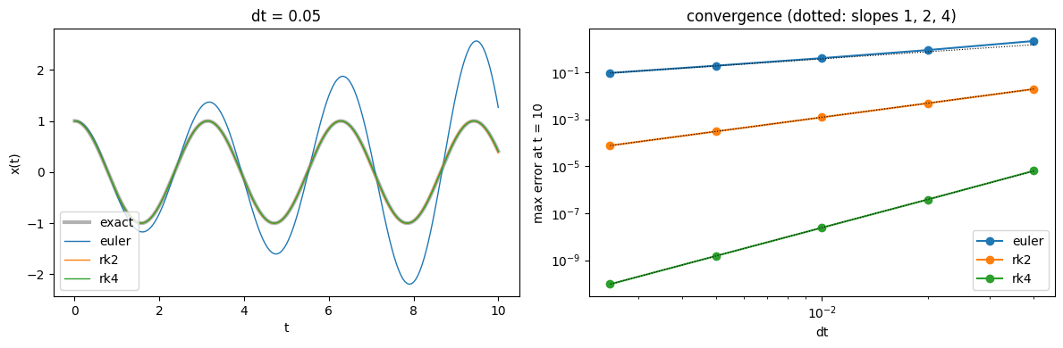
RK2 and RK4 converge at their nominal orders 2 and 4 from the start: halving dt divides the error by 4 and 16. Euler approaches order 1 only slowly (observed orders 1.28 down to 1.03), because on an oscillator it multiplies the amplitude by \(\sqrt{1 + \omega^2 \Delta t^2}\) every step: at dt = 0.05 its trajectory spirals outward, and at dt = 0.04 its final error (2.15) exceeds the amplitude of the solution. RK4 at dt = 0.04 (error 6.4e-6) is about 10,000 times more accurate than Euler with a 16 times smaller step (error 0.09 at dt = 0.0025).
2. Adaptive steps with solve_ivp#
A fixed step must be small enough for the fastest part of the trajectory everywhere. The Van der Pol oscillator
with \(\mu = 10\) is a relaxation oscillator: slow drifts alternate with fast jumps. That makes it stiff-ish, and the right step size varies by orders of magnitude along the cycle. solve_ivp uses an embedded Runge–Kutta pair ('dopri5', Dormand–Prince 5(4), by default): each step also yields an error estimate, the step is accepted when the error is below atol + rtol * |y|, and a PI controller picks the next step size.
Without t_eval, the solution holds the accepted steps. The output has a static length of max_steps + 1 (here the default 4096 + 1), padded after the n_steps accepted steps:
def van_der_pol(y, t, mu):
    x, v = y
    return jnp.stack([v, mu * (1 - x ** 2) * v - x])


mu = 10.0
vdp_y0 = jnp.array([2.0, 0.0])
t_span = (0.0, 40.0)

sol = quad.solve_ivp(van_der_pol, t_span, vdp_y0, mu, rtol=1e-6, atol=1e-9)
n = int(sol.n_steps)
print(f'accepted steps: {n}, rejected: {int(sol.n_rejected)}, success: {bool(sol.success)}')
print('output length:', sol.ts.shape[0], ' last time:', float(sol.ts[n]))
h = np.diff(np.asarray(sol.ts[:n + 1]))
print(f'step size: min {h.min():.2e}, max {h.max():.2e}')
accepted steps: 859, rejected: 15, success: True
output length: 4097  last time: 40.0
step size: min 5.00e-04, max 8.32e-02
SciPy’s solve_ivp with its own Dormand–Prince pair ('RK45') at the same tolerances takes a similar number of steps. The counts differ somewhat because the step-size controllers differ (braintools uses a PI controller, SciPy a plain one):
def van_der_pol_scipy(t, y):
    return [y[1], mu * (1 - y[0] ** 2) * y[1] - y[0]]


sp = scipy.integrate.solve_ivp(van_der_pol_scipy, t_span, np.asarray(vdp_y0), method='RK45', rtol=1e-6, atol=1e-9)
print(f'scipy RK45: accepted steps {len(sp.t) - 1}, function evaluations {sp.nfev}, success {sp.success}')
scipy RK45: accepted steps 691, function evaluations 4490, success True
fig, axes = plt.subplots(2, 1, figsize=(10, 5), sharex=True)
axes[0].plot(sol.ts[:n + 1], sol.ys[:n + 1, 0], '.-', ms=2, lw=0.8)
axes[0].set_ylabel('x(t)')
axes[0].set_title(f'Van der Pol, mu = {mu:g}: {n} accepted dopri5 steps')
axes[1].semilogy(sol.ts[1:n + 1], h, lw=0.8)
axes[1].set_ylabel('step size')
axes[1].set_xlabel('t')
plt.tight_layout()
plt.show()
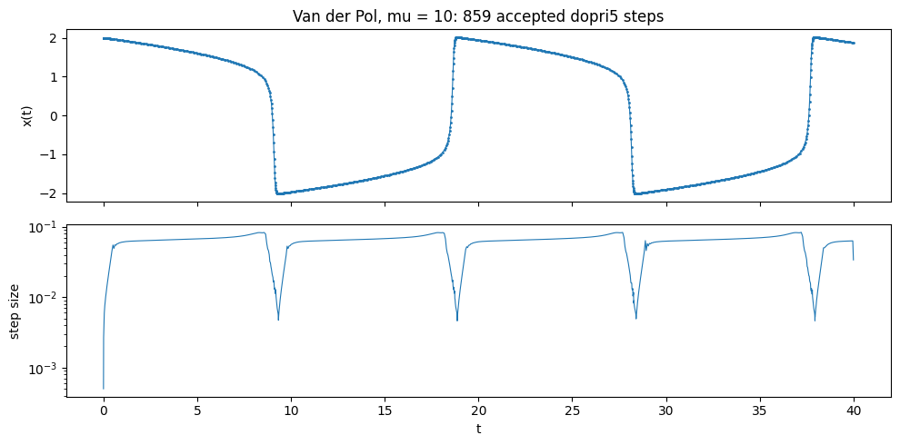
The first step is small (the starting-step heuristic picks 5e-4). After that, the step size grows to about 0.08 on the slow branches and drops more than tenfold, to about 0.005, during each fast jump of \(x\).
Output at requested times: t_eval#
With t_eval, the solution is returned at the requested times. solve_ivp shortens any step that would cross a t_eval point so that it lands on it, so the outputs have the accuracy of the solver itself rather than of an interpolant. This costs about one extra step per output point. Below, both solvers return 401 points; the reference is SciPy’s 8th-order 'DOP853' at rtol = atol = 1e-12:
t_eval = jnp.linspace(*t_span, 401)

start = time.perf_counter()
sol_te = quad.solve_ivp(van_der_pol, t_span, vdp_y0, mu, rtol=1e-6, atol=1e-9, t_eval=t_eval)
jax.block_until_ready(sol_te.ys)
print(f'braintools dopri5: accepted steps {int(sol_te.n_steps)}, rejected {int(sol_te.n_rejected)} '
      f'(compile + run {time.perf_counter() - start:.1f} s)')

sp_te = scipy.integrate.solve_ivp(van_der_pol_scipy, t_span, np.asarray(vdp_y0), method='RK45',
                                  rtol=1e-6, atol=1e-9, t_eval=np.asarray(t_eval))
ref = scipy.integrate.solve_ivp(van_der_pol_scipy, t_span, np.asarray(vdp_y0), method='DOP853',
                                rtol=1e-12, atol=1e-12, t_eval=np.asarray(t_eval))

err_bt = np.abs(np.asarray(sol_te.ys[:, 0]) - ref.y[0])
err_sp = np.abs(sp_te.y[0] - ref.y[0])
print(f'max |x - reference|: braintools {err_bt.max():.1e}, scipy RK45 {err_sp.max():.1e}')

plt.figure(figsize=(10, 3))
plt.semilogy(t_eval, err_bt + 1e-16, lw=0.8, label='braintools dopri5')
plt.semilogy(t_eval, err_sp + 1e-16, lw=0.8, label='scipy RK45 (dense output)')
plt.xlabel('t')
plt.ylabel('|x - reference|')
plt.title('error at the 401 t_eval points (rtol=1e-6, atol=1e-9)')
plt.legend()
plt.tight_layout()
plt.show()
braintools dopri5: accepted steps 1449, rejected 3 (compile + run 1.1 s)
max |x - reference|: braintools 5.0e-05, scipy RK45 1.7e-04
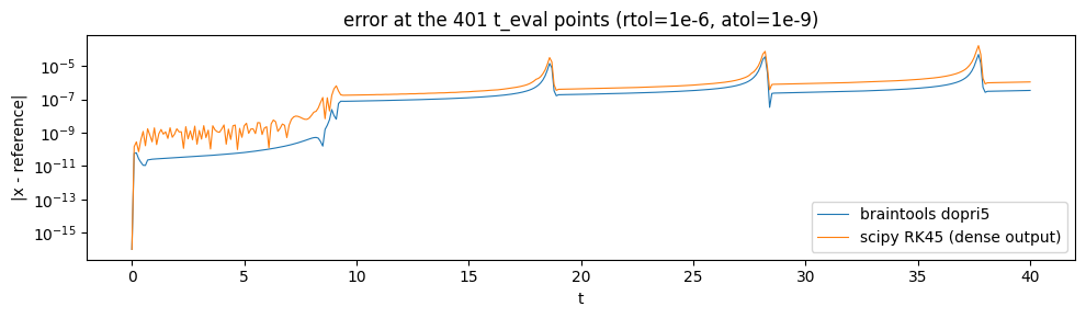
The maximum errors are 5.0e-5 for braintools and 1.7e-4 for SciPy. For both, the error jumps at each fast transition of \(x\), where a small error in the timing of the jump becomes a large difference in \(x\). SciPy interpolates its dense output at t_eval; braintools instead steps onto every output time. That costs extra steps (1449 accepted steps with t_eval against 859 without), but the outputs are as accurate as the steps themselves.
The method argument selects other embedded pairs. A higher-order pair takes fewer, more expensive steps at tight tolerances:
for m in ['rk23', 'dopri5', 'dopri8']:
    s = quad.solve_ivp(van_der_pol, t_span, vdp_y0, mu, method=m, rtol=1e-8, atol=1e-10, t_eval=t_eval)
    err = np.abs(np.asarray(s.ys[:, 0]) - ref.y[0]).max()
    print(f'{m:7s} accepted {int(s.n_steps):5d}  rejected {int(s.n_rejected):4d}  '
          f'max error {err:.1e}  success {bool(s.success)}')
rk23 accepted 4096 rejected 0 max error 3.9e+00 success False
dopri5 accepted 2632 rejected 0 max error 3.6e-07 success True
dopri8 accepted 1173 rejected 9 max error 8.9e-09 success True
At rtol = 1e-8, the 8th-order 'dopri8' (DOP853) needs fewer than half the steps of 'dopri5' (1173 against 2632) and is more accurate. The third-order 'rk23' would need far more steps than either: it uses up the default max_steps = 4096 attempts before reaching t1 = 40, so success is False. The outputs after the last accepted step hold that step’s state, hence the large error. Raise max_steps (a static size, which costs compile time and memory) or use a higher-order pair.
3. Gradients through the solvers#
Both drivers are differentiable with respect to the initial state, the extra arguments and the times. A common use is a parameter sensitivity: how much the trajectory changes when a parameter changes. Below, jax.jacfwd gives \(\partial x(t) / \partial \mu\) at all 201 output times of a Van der Pol oscillator with \(\mu = 1\), checked against a central finite difference.
t_sens = jnp.linspace(0.0, 20.0, 201)


def x_traj(mu):
    s = quad.solve_ivp(van_der_pol, (0.0, 20.0), vdp_y0, mu, rtol=1e-10, atol=1e-12, t_eval=t_sens)
    return s.ys[:, 0]


sens = jax.jacfwd(x_traj)(1.0)
eps = 1e-5
sens_fd = (x_traj(1.0 + eps) - x_traj(1.0 - eps)) / (2 * eps)
print('dx(t)/dmu:', sens.shape, f' max |AD - finite difference| = {float(jnp.max(jnp.abs(sens - sens_fd))):.1e}')

fig, axes = plt.subplots(2, 1, figsize=(10, 4.5), sharex=True)
axes[0].plot(t_sens, x_traj(1.0), label='mu = 1')
axes[0].plot(t_sens, x_traj(1.2), '--', label='mu = 1.2')
axes[0].set_ylabel('x(t)')
axes[0].legend(loc='upper right')
axes[1].plot(t_sens, sens, label='jax.jacfwd')
axes[1].plot(t_sens[::5], sens_fd[::5], 'k.', ms=4, label='finite difference')
axes[1].set_ylabel('dx(t) / dmu')
axes[1].set_xlabel('t')
axes[1].legend(loc='upper left')
plt.tight_layout()
plt.show()
dx(t)/dmu: (201,) max |AD - finite difference| = 2.4e-07
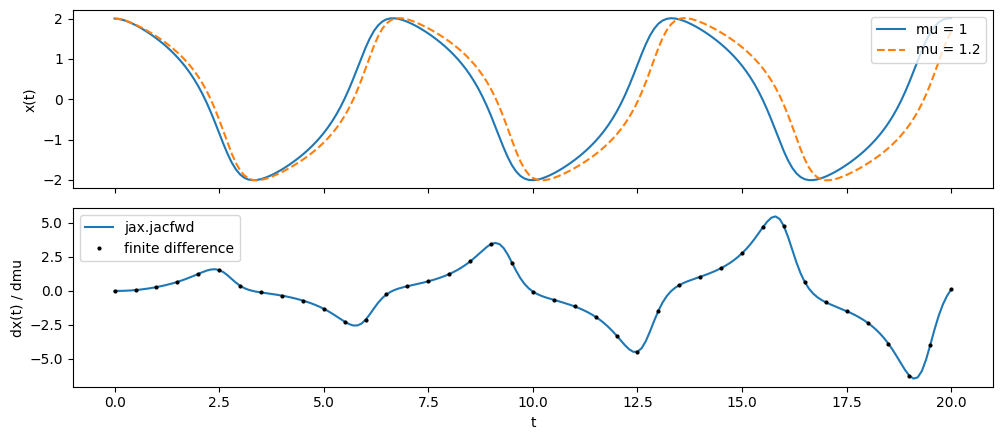
A larger \(\mu\) lengthens the period, so the phase lag accumulates from cycle to cycle and the sensitivity oscillates with growing amplitude. The automatic derivative matches the finite difference to 2.4e-7.
Reverse mode (jax.grad) is what training and fitting use. It must keep the intermediate states of the forward pass, which for long rollouts can exhaust memory. checkpoint=True stores only some of them and recomputes the rest on the backward pass, so memory no longer grows with the number of steps; the values and gradients are the same. It is the default for solve_ivp (whose loop always has max_steps iterations) and opt-in for odeint:
def loss_odeint(omega, checkpoint):
    _, ys = quad.odeint(oscillator, y0, 0.0, 50.0, 0.001, omega, checkpoint=checkpoint)  # 50,000 steps
    return jnp.mean(ys[:, 0] ** 2)


def loss_ivp(mu, checkpoint):
    s = quad.solve_ivp(van_der_pol, (0.0, 20.0), vdp_y0, mu, rtol=1e-8, atol=1e-10,
                       t_eval=t_sens, checkpoint=checkpoint)
    return jnp.mean(s.ys[:, 0] ** 2)


for name, loss, p in [('odeint', loss_odeint, omega), ('solve_ivp', loss_ivp, 1.0)]:
    g_plain = jax.grad(loss)(p, False)
    g_ckpt = jax.grad(loss)(p, True)
    g_fd = (loss(p + eps, False) - loss(p - eps, False)) / (2 * eps)
    print(f'{name:9s} grad (checkpoint=False) {float(g_plain):+.8f}   (checkpoint=True) {float(g_ckpt):+.8f}'
          f'   finite difference {float(g_fd):+.8f}')
odeint grad (checkpoint=False) +0.12332256 (checkpoint=True) +0.12332256 finite difference +0.12332254
solve_ivp grad (checkpoint=False) -0.10313317 (checkpoint=True) -0.10313317 finite difference -0.10313316
solve_ivp treats the accepted step sizes as constants when differentiating (“discretise, then optimise”), so its gradient is the exact gradient of the computed solution, and it agrees with the finite difference to the accuracy of the solve.
4. The method registry#
odeint and solve_ivp look their method up in a registry of steppers, one table per equation kind ('ode', 'sde', 'imex', 'dde'). list_methods lists the names, and get_method returns the stepper; the full function name works too:
print('ODE methods:', quad.list_methods('ode'))
print('SDE methods:', quad.list_methods('sde'))
print("get_method('rk4') is ode_rk4_step:", quad.get_method('rk4') is quad.ode_rk4_step)
print("get_method('ode_dopri5_step') is ode_dopri5_step:", quad.get_method('ode_dopri5_step') is quad.ode_dopri5_step)
try:
    quad.get_method('rk5')
except KeyError as e:
    print('KeyError:', e)
ODE methods: ['bs32', 'dopri5', 'dopri8', 'euler', 'expeuler', 'heun', 'midpoint', 'ralston2', 'ralston3', 'rk2', 'rk23', 'rk3', 'rk4', 'rk45', 'rk45_dopri', 'rk4_38', 'rk87_dopri', 'rkf45', 'ssprk33']
SDE methods: ['euler', 'expeuler', 'heun', 'implicit_euler', 'milstein', 'srk2', 'srk3', 'srk4', 'tamed_euler']
get_method('rk4') is ode_rk4_step: True
get_method('ode_dopri5_step') is ode_dopri5_step: True
KeyError: "Unknown 'ode' method 'rk5'. Did you mean one of ['rk45', 'rkf45', 'rk4', 'rk3', 'rk2']? Available methods: ['bs32', 'dopri5', 'dopri8', 'euler', 'expeuler', 'heun', 'midpoint', 'ralston2', 'ralston3', 'rk2', 'rk23', 'rk3', 'rk4', 'rk45', 'rk45_dopri', 'rk4_38', 'rk87_dopri', 'rkf45', 'ssprk33']."
register_method(name, fn) adds a stepper. It must follow the convention of the built-in ODE steppers: fn(f, y, t, *args, **kwargs) returns the state after one step, with the step size read from brainstate.environ.get_dt() (odeint sets it from its dt argument).
As an example, the function below builds an explicit Runge–Kutta stepper from a Butcher tableau, and registers Kutta’s classical third-order method under the name 'kutta3'. overwrite=True lets the cell run twice; without it, registering an existing name raises ValueError. Once registered, odeint accepts the new name, and the convergence study of section 1 confirms the order:
def make_explicit_rk(a, b, c):
    """Return an ODE stepper for the explicit Runge-Kutta tableau (a, b, c)."""

    def step(f, y, t, *args, **kwargs):
        dt = brainstate.environ.get_dt()
        ks = []
        for i in range(len(b)):  # loop over the stages of one step (unrolled at trace time)
            yi = y + dt * sum(a[i][j] * ks[j] for j in range(i)) if i else y
            ks.append(f(yi, t + c[i] * dt, *args, **kwargs))
        return y + dt * sum(bi * k for bi, k in zip(b, ks))

    return step


kutta3 = make_explicit_rk(a=[[], [1 / 2], [-1, 2]], b=[1 / 6, 2 / 3, 1 / 6], c=[0, 1 / 2, 1])
quad.register_method('kutta3', kutta3, overwrite=True)
print("'kutta3' registered:", 'kutta3' in quad.list_methods('ode'))

err_k3 = np.array([float(jnp.max(jnp.abs(quad.odeint(oscillator, y0, 0.0, T, dt, omega, method='kutta3')[1][-1]
                                         - exact_T)))
                   for dt in dts])
print('kutta3 errors', np.array2string(err_k3, precision=2),
      ' observed order', np.round(np.log2(err_k3[:-1] / err_k3[1:]), 2))
'kutta3' registered: True
kutta3 errors [7.55e-04 9.59e-05 1.21e-05 1.52e-06 1.90e-07] observed order [2.98 2.99 2.99 3. ]
Halving the step divides the error by about 8, as expected for a third-order method. The stage loop inside the stepper is a plain Python loop over the three stages of one step: it is unrolled when odeint traces the stepper once, while the loop over time steps stays inside the compiled scan.
solve_ivp additionally needs an error estimate and the order of that estimate for its step-size controller, so it accepts only the built-in embedded pairs, which the error message lists. A registered stepper such as 'kutta3' works with odeint but is rejected by solve_ivp with a ValueError:
try:
    quad.solve_ivp(oscillator, (0.0, 1.0), y0, omega, method='kutta3')
except ValueError as e:
    print('ValueError:', e)
ValueError: Method 'kutta3' has no embedded error estimate. Adaptive methods: ['bs32', 'dopri5', 'dopri8', 'rk23', 'rk45', 'rk45_dopri', 'rk87_dopri', 'rkf45'].
For the single-step functions behind these drivers, see the ODE, SDE and IMEX and delay tutorials; for fitting models with odeint and solve_ivp, the model-fitting tutorial; and for every parameter, the API reference.